The fundamental goal of inventory control is to guarantee that sufficient items or resources are available to fulfill demand without generating surplus inventory. That brings us to the following lesson – creating a step-by-step process for establishing the Min Max Inventory Calculation in Excel.
Key Stock Level Metrics in an Inventory System?
- Safety Stock
Safety Stock = [Maximum Consumption * Maximum Delivery Time] – [Average Consumption * Average Delivery Time]
- Order Quantity
Order Quantity = Damages + Safety Stock
- Min Inventory Level
Minimum Inventory level = Order Quantity – [Average Consumption × Average Delivery Time]
- Max Inventory Level
Maximum Inventory Level = Safety Stock + Order Quantity – [Minimum Consumption * Minimum Delivery Time]
Min Max Inventory Calculation in Excel: With Easy Steps
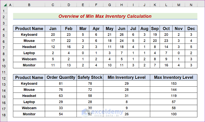
The below dataset has a column titled Product Name that contains some computer accessories, and other columns keep information about their monthly sales from January to December. We will determine the necessary Order Quantity and Safety Stock throughout the following steps. With the help of two typical formulas, we will also establish the Min Max Inventory Calculation.
Make sure you download the sheet from the practice workbook linked below when using these methods.
Method 1 – Use a Date Model to Calculate Min Max Inventory in Excel
- Select the DemandSupply sheet.
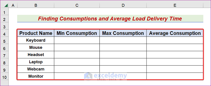
- Highlight the four columns titled Product Name, Min Consumption, Max Consumption, and Average Consumption.
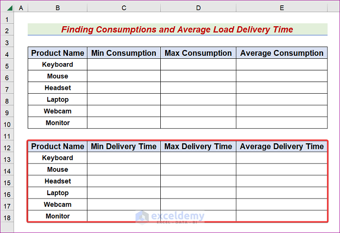
- Make another table for the Delivery Time in the B12:E18 range.
- Open the SafetyStock sheet.
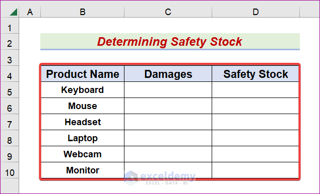
- Select three columns: Product Name, Damages, and Safety Stock.
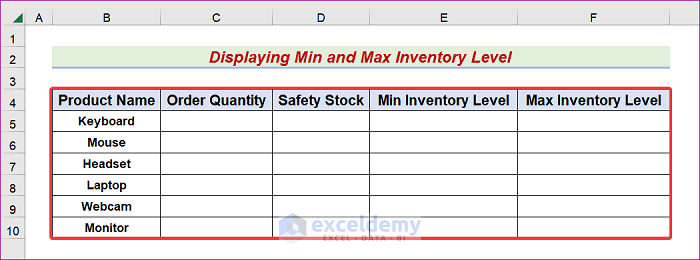
- Choose the B4:F10 range to display the Min Max Inventory Level.
Read More: How to Keep Track of Inventory in Excel
Method 2 – Apply MIN, MAX, ROUND and AVERAGE Functions to Get Consumptions of Inventory
The MIN function finds the lowest digit in a list. Meanwhile, the MAX function multiplies together the most significant value in a collection. The ROUND function in Excel provides a result rounded to a specified precision. The AVERAGE function finds the average of the numbers you provide. The Consumption data will be determined using these procedures.
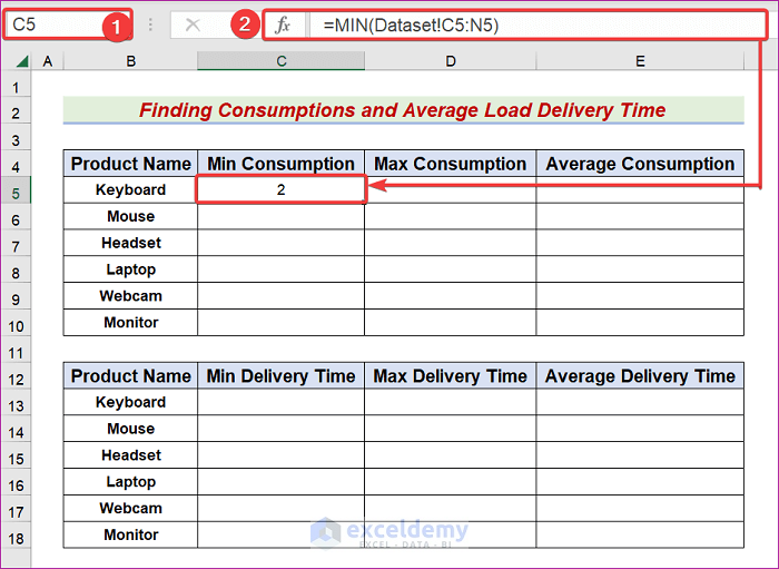
- Open the DemandSupply sheet and select the C5 cell.
- Input the following equation in the Formula bar.
=MIN(Dataset!C5:N5)
- Press the Enter or Tab key to see the result.
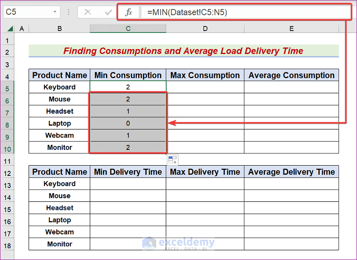
- Drag the AutoFill Handle to cell C10 to apply the same formula to other cells in the Min Consumption column.
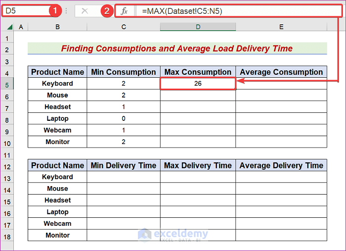
- Choose cell D5.
- Type for following in the Formula bar.
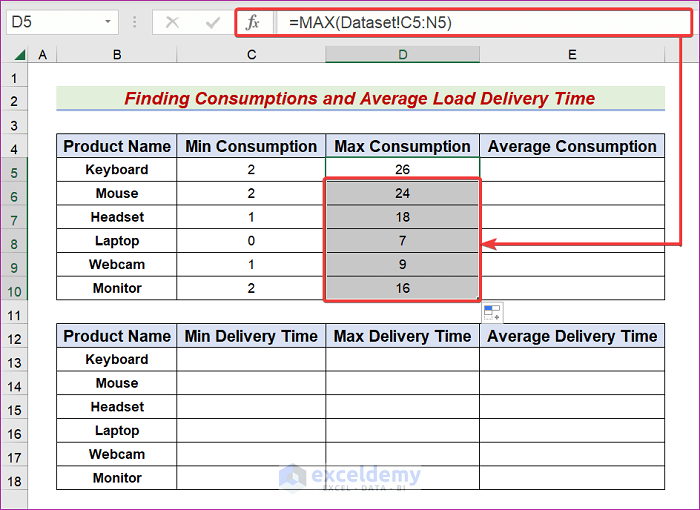
=MAX(Dataset!C5:N5)
- Press the Enter or Tab key to see the result.
- Drag the AutoFill Handle to cell D10 to apply the same equation to other cells in the Max Consumption section.
- Choose cell E5.
- Type the following equation into the Formula bar.
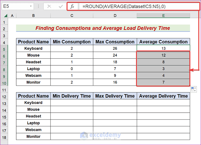
=ROUND(AVERAGE(Dataset!C5:N5),0)
- Press the Enter or Tab key to see the result.

- You can also use the AutoFill Handle icon to apply the same formula to other cells in the Average Consumption portion.
=MIN(Dataset!C5:N5)
To understand this formula, you must be familiar with the following Excel function:
MIN Function
- MIN(Dataset!C5:N5)
The MIN function finds the least significant digit in a list. Enter an Exclamation mark between the sheet’s name and the range to refer to data or cells in other sheets. In this example, by involving the MIN function, we find 2.
=MAX(Dataset!C5:N5)
For this formula to make sense, you need to know how to use the following Excel function:
MAX Function
- MAX(Dataset!C5:N5)
When called, the MAX function always returns the highest number in the given range. In this example, by using the MAX function, we get 26.
=ROUND(AVERAGE(Dataset!C5:N5),0)
To understand this formula, you must be familiar with the following Excel function:
ROUND and AVERAGE Functions
- AVERAGE(Dataset!C5:N5)
In Excel, you can get the mean of a set of integers using the AVERAGE function. To refer to data or cells in other sheets, you must use an Exclamation sign between the sheet name and range. In this demonstration, by involving the AVERAGE function, we find 12.8333333333333.
- ROUND(AVERAGE(Dataset!C5:N5),0)
The ROUND function is what we need to round off a value to a certain precision. In this context, by utilizing the Round function, we find 13.
Read More: How to Maintain Store Inventory in Excel
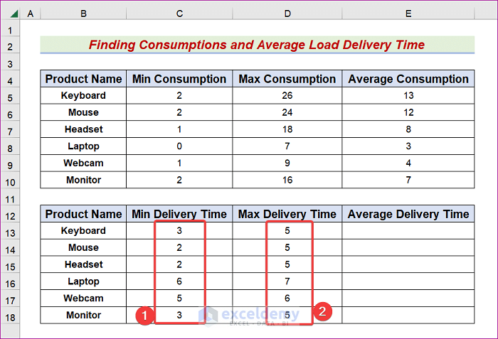
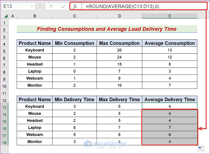
Method 3 – Use the AVERAGE Function to Find Average Load Time of Inventory in Excel
- Input the Min and Max Delivery Time throughout the C and D columns.
- Select cell E13.
- Type the following equation into the Formula bar:
=ROUND(AVERAGE(C13:D13),0)
- Press the Enter or Tab key to see the result.
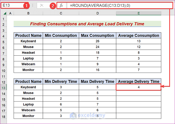
- Use the AutoFill Handle to apply the same formula to other cells in the Average Delivery Time column.
Read More: How to Make Inventory Aging Report in Excel
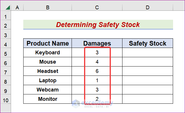
Method 4 – Determine Safety Stock for Min Max Inventory Calculation
- Open the SafetyStock sheet.
- Input the intended values in the Damages column.
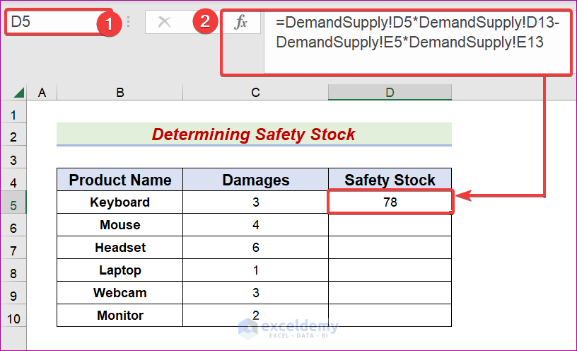
- Select cell D5.
- Type this equation into the Formula bar.
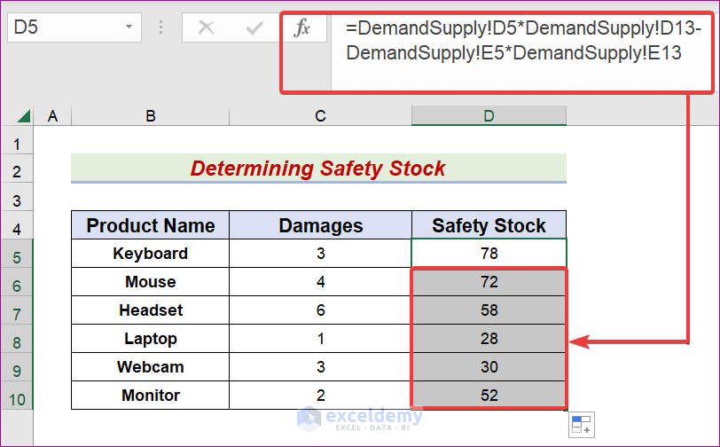
=DemandSupply!D5*DemandSupply!D13-DemandSupply!E5*DemandSupply!E13
- Press Enter or Tab to see the result.
- Drag the AutoFill Handle to apply the same formula to other cells in the Safety Stock column.
Read More: How to Create Inventory Database in Excel
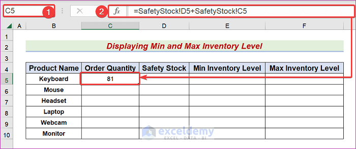
Method 5 – Display Min Max Inventory Calculation in Excel
- Choose the C5 cell in the Min Max Inventory sheet.
- Type the following equation into the Formula bar.
=SafetyStock!D5+SafetyStock!C5
- See the result using the Enter or Tab key.
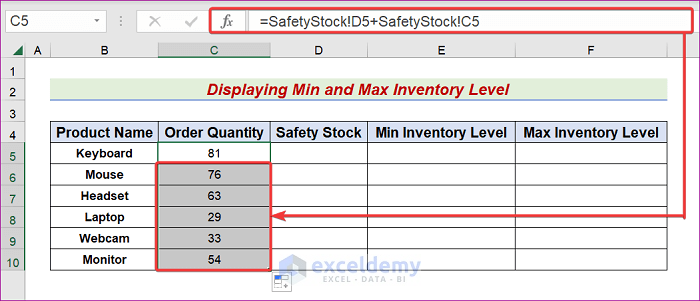
- Drag the AutoFill Handle icon to C10 to apply the same formula to more cells in the Order Quantity section.
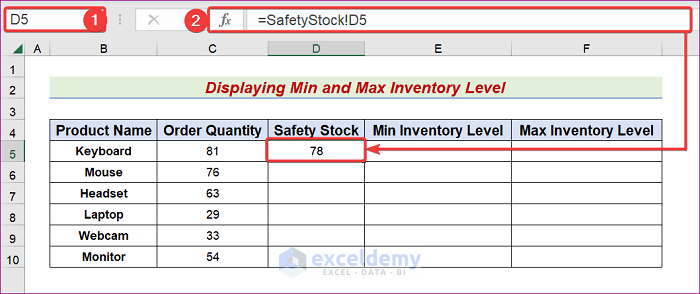
- Highlight cell D5.
- Enter the following in the Formula bar.
=SafetyStock!D5
- Tap the Enter or Tab key to see your result.
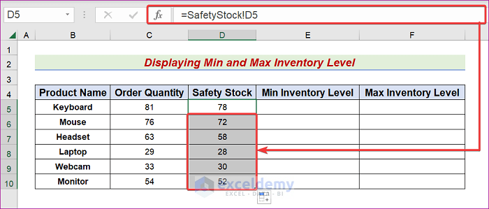
- Use the AutoFill Handle icon to apply the same formula to other cells in the Safety Stock section.
- Select cell E5.
- Enter the following formula in the Formula bar.
=C5-DemandSupply!E5*DemandSupply!E13
- Use the Enter or Tab key to retrieve the result.
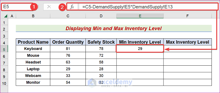
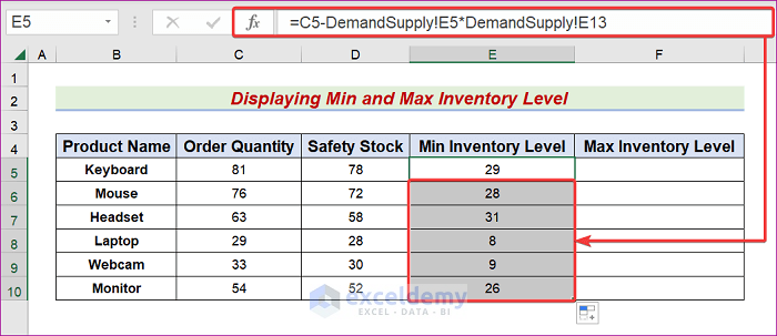
- Use the AutoFill Handle icon to apply the same procedure to other cells within the Minimum Inventory Level.
- Go to cell F5.
- Copy and paste this formula into the Formula bar.
=D5+C5-DemandSupply!C5*DemandSupply!C13
- Hit Enter or Tab to see the output.
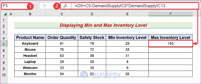
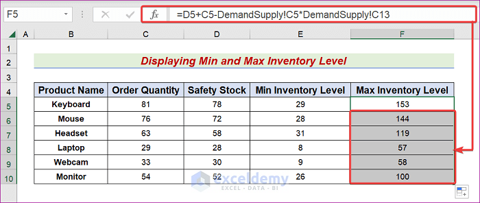
- Drag AutoFill Handle symbol to cell F10.
- You should see the following output displayed in your table.
Download Practice Workbook
If you want a free copy of the sample workbook covered during the presentation, kindly click the link below this paragraph.
Related Articles
- How to Calculate Economic Order Quantity in Excel
- How to Calculate Stock to Sales Ratio Using Formula in Excel
<< Go Back to Inventory Management in Excel | Learn Excel
Get FREE Advanced Excel Exercises with Solutions!

Mantap, terima kasih banyak
Hello Dear,
Sama-sama. Thanks for your appreciation and feedback. Keep exploring Excel with ExcelDemy!
Regards
ExcelDemy