Basic Overview of the Steps:
- Specify the most important criteria related to the process.
- Assign a weight to each criterion. The summation of the weights should be 100%.
- Assign scores to the options.
- You need to find the weighted scores. To do so, multiply the weight for each criterion by its score and add them up.
How to Create a Weighted Scoring Model in Excel: 4 Examples
Example 1 – Choose the Best Location by Creating a Weighted Scoring Model in Excel
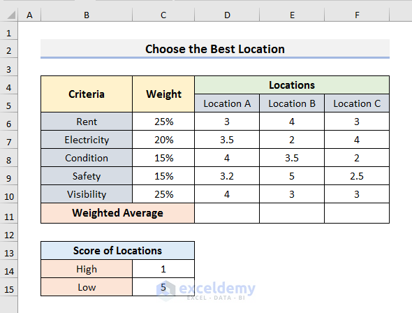
We will choose the best location for setting up a production house by creating a weighted scoring model in Excel. We have assigned the criteria and their weights in the dataset below. We have included the numerical scores between 1 to 5 for locations A, B, and C. We will calculate the weighted average score.
STEPS:
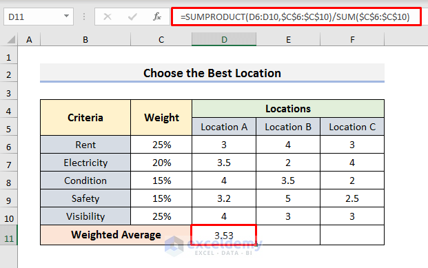
- Select Cell D11 and use this formula:
=SUMPRODUCT(D6:D10,$C$6:$C$10)/SUM($C$6:$C$10)- Hit Enter to see the result.
- Drag the Fill Handle to the right to see results for Locations B and C.
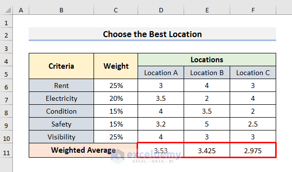
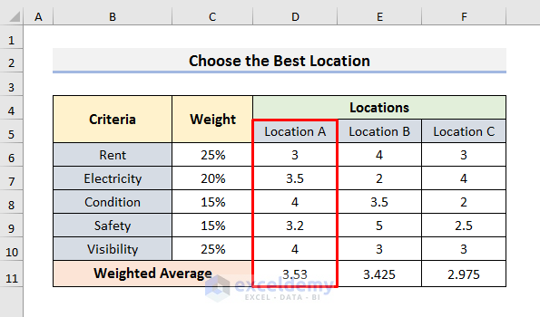
- Location A is the best option for setting up a production house as it scores the highest.
Note: To determine the weighted score without average, use the formula below:
=SUMPRODUCT(D6:D10,$C$6:$C$10)How Does the Formula Work?
- SUMPRODUCT(D6:D10,$C$6:$C$10)
This part of the formula calculates the product for each criterion and then adds them up. Generally, it represents the basic formula,
D6*C6+D7*C7+D8*C8+D9*C9+D10*C10
- SUM($C$6:$C$10)
Here, this part computes the sum of the range C6:C10.
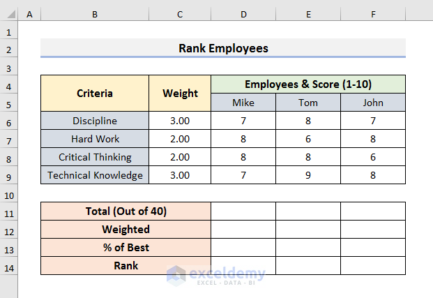
Example 2 – Design a Weighted Scoring Model to Rank Employees
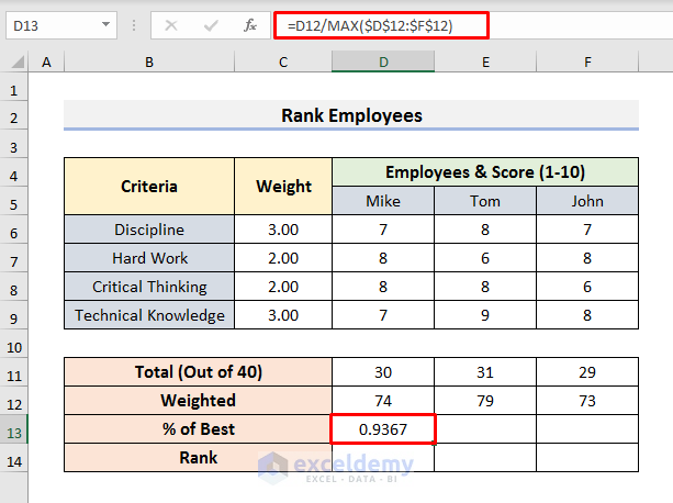
We have assigned 4 criteria. The weights of these criteria sum up to 10. The scores of the employees are also distributed.
STEPS:
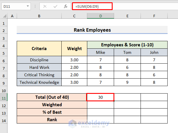
- Select Cell D11 and use the SUM formula:
=SUM(D6:D9)- Press Enter to see the result.
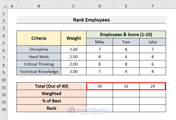
- Drag the Fill Handle to the right.
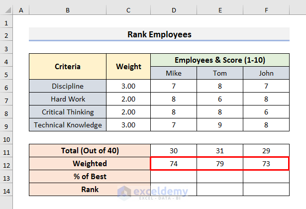
- Select Cell D12 and use the following formula:
=SUMPRODUCT(D6:D9,$C$6:$C$9)- Hit Enter to see the result.

- Use the Fill Handle in Row 12 for the rest of the cells.
- Select Cell D13 and insert this formula:
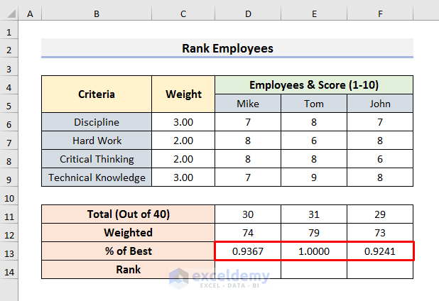
=D12/MAX($D$12:$F$12)- Press Enter to see the result.
- Drag the Fill Handle to the right.
- Select Cell D14 and insert the formula:
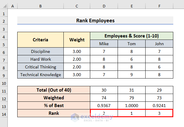
=RANK(D13,$D$13:$F$13)- Hit Enter.
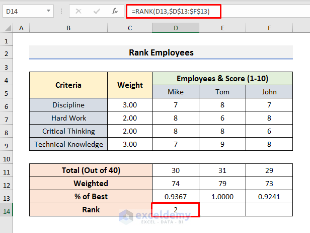
- Use the Fill Handle to rank the employees. We can see Tom ranks first.
Example 3 – Generate a Weighted Scoring Model in Excel and Determine the Highest Priority
We have 3 requirements and need to find which requirement should get the highest priority.
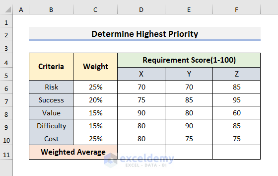
STEPS:
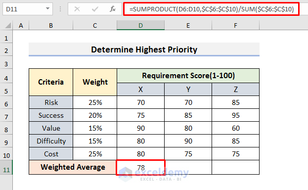
- Select Cell D11 and insert this formula:
=SUMPRODUCT(D6:D10,$C$6:$C$10)/SUM($C$6:$C$10)- Press Enter to see the result.
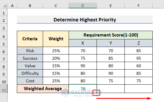
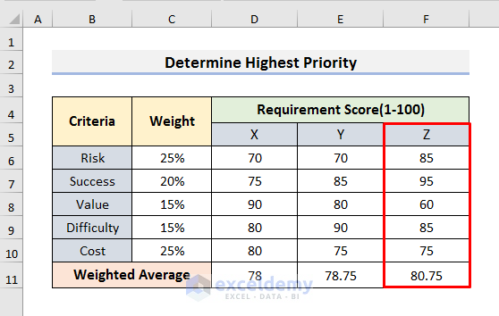
- Drag the Fill Handle to the right to copy the formula.
- You will get the results. Requirement Z should get the highest priority.
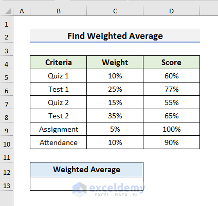
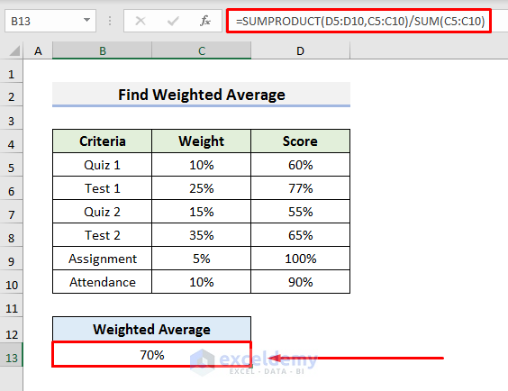
Example 4 – Find the Weighted Average by Creating a Scoring Model in Excel
A student has attended some quizzes, exams, and assignments. At the end of the year, we need to calculate his weighted average marks. We can see the weights of the exams and the scores in percentage. The quizzes, exams, assignments, and attendance are the criteria here.
STEPS:
- Select Cell B13.
- Insert the following formula:
=SUMPRODUCT(D5:D10,C5:C10)/SUM(C5:C10)- Press Enter to see the weighted average marks.
Things to Remember
- Don’t forget to use absolute reference. If you don’t use absolute references, then, you will get incorrect results or errors when copying or using AutoFill.
- Assign the criteria carefully.
- The weights can be assigned in numerical values or percentages.
Download the Practice Book
<< Go Back to Scoring | Formula List | Learn Excel
Get FREE Advanced Excel Exercises with Solutions!
