Timesheet Formula in Excel (5 Examples)

To calculate the time difference (e.g. work hours) between two time periods, we create a timesheet. There are several ways that we can use to keep track of time on a timesheet. Using formulas in Excel timesheets can make it easier and more convenient to apply. In this regard, this article will help you learn the timesheet formula in Excel with 5 relevant examples.

How to Timesheet Formula in Excel: 5 Examples

Let’s assume that we have a data table, Employee Work Hour Timesheet. We will use this dataset to demonstrate all the examples regarding the timesheet formula in Excel one by one.

1. Excel Timesheet Formula: Using Simple Subtraction

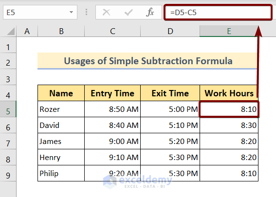
We have a worksheet of four columns data table. The data table stores the entry and exit time of employees and calculates their total work hours on a daily basis. The first column stores employee names, the second column holds entry time, the third column contains exit time, and the last column keeps the work hours count.

Now we can apply the simple arithmetic subtraction formula within this Excel timesheet. To do that, follow the steps below:

❶ First of all type of formula is below within cell E5.

❷ After that press the ENTER button to execute the subtraction formula.

❸ Finally drag the Fill Handle icon to the end of the Work Hours column.

2. Excel Timesheet Formula: Using MOD Function

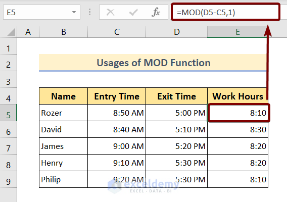
Instead of using the simple arithmetic subtraction formula, we can use the MOD function to do so. Actually, we will use the subtraction formula inside the MOD function, within its argument list.

The MOD function has two arguments in total. In place of the first argument, we will insert the subtraction formula, and the second argument requires a divider value. Which will be 1 for this instance.

Now follow the steps below to learn the procedure:

❶ Select cell E5 to insert the formula below:

❷ After that, press the ENTER button.

❸ Lastly, drag the Fill Handle icon to the end of the Work Hours column.

That’s all.

3. Excel Timesheet Formula: Using MOD Function Considering Break

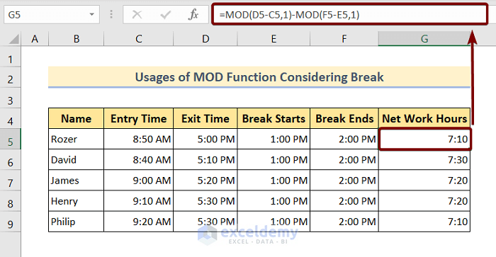
In this second, we will again apply the MOD function into the timesheet Excel formula. But this time we will consider the work break to calculate the Net Work Hours by each of the employees.

To calculate the Net Work Hours, we must subtract the break period from the total office time period. So, we will use two MOD functions in total.

The first MOD function will return the total office work period, whereas the second MOD function will return the total break period. By subtracting these two results, we can easily get the Net Work Hours by each of the employees.

Now follow the steps below to learn it step by step:

❶ Type the timesheet formula below within cell G5.

❷  Now press the ENTER button.

❸ At the end, draw the Fill Handle icon to the end of the Net Work Hours column.

4. Excel Timesheet Formula: Using Simple Addition Formula

This time we will calculate the total work hours in a different way. We will use the simple arithmetic addition formula to calculate the work hours of each of the employees.

So, we’ve divided the work hour count into two categories. Those are total work hours before the break and again total work hours after the break.

Now we can calculate the total work hours simply by adding work hours before the break to the work hours after the break.

To do that, follow the steps below:

❶ At first type the formula below within cell E5.

❷ Then press the ENTER button.

❸ Finally, pull the Fill Handle icon to the bottom of the Work Hours column.

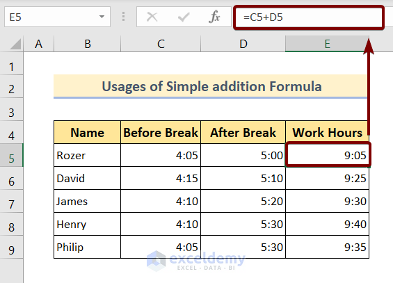
That’s it.

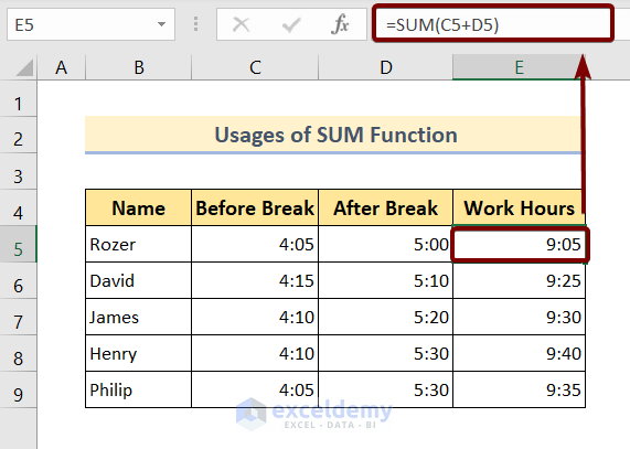
5. Excel Timesheet Formula: Using SUM Function

Now instead of using the simple addition formula, we will use the SUM function. Well, here one thing is to mention. That is though both of the formulas serve the same purpose, still, there’s a difference.

When there is only a little cell reference to add, then we can use either the simple addition formula or the formula with the SUM function.

But when you have to sum up a large number of cell references, then there’s no alternative to using the SUM function.

Now, follow the steps below to do that,

❶ Select cell E5 and type the formula below:

❷ Press the ENTER button.

❸ Draw the Fill Handle icon to the end of the Work Hours column.

Things to Remember

📌 As you are working with the timesheet, always set the cell format to Time.

Download the Practice Workbook

You can download the Excel file from the link below and practice along with it.

Conclusion

To sum up, we have discussed 5 relevant examples to demonstrate the usage of the timesheet formula in Excel. You are recommended to download the practice workbook attached along with this article and practice all the methods with that. And don’t hesitate to ask any questions in the comment section below. We will try to respond to all the relevant queries asap.

Ageing Formula in Excel: Knowledge Hub

<< Go Back to Formula List | Learn Excel