Do you urgently require an Employee Timesheet? You’ve found the right place if the response is yes. Excel makes it very easy to manage and track work hours. In this article, we will take you through 5 easy and quick steps on how to create an employee Timesheet in Excel.
How to Create an Employee Timesheet in Excel: Step-by-Step Procedure
Generally speaking, the HR department of an organization manages Timesheets that involve recording and evaluating employee timekeeping. Additionally, it may entail performing various tasks, such as calculating employee payroll. So, without further delay, let’s see the process of creating an employee timesheet in Excel in detail.
Step 1: Prepare Basic Information Structure
Here, we’re showing the full process in different steps so that it is easy to understand. To make it easier to understand, we break down the entire process into its component parts here. First of all, we need to create a basic outline of the monthly worksheet. So, just follow along.
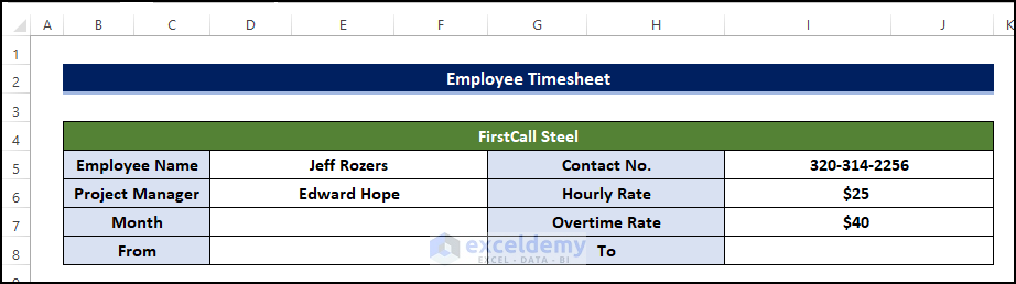
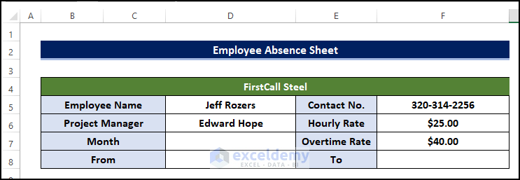
- In cell B4, write down the name of the company. Here, we assumed it FirstCall Steel.
- Also, place the Employee Name, Project Manager’s name, Contact No, Hourly Rate, and Overtime Rate.
Step 2: Input Basic Information of Employee for Timesheet
In the next step, we will formalize the information to make it more dynamic and user-friendly. The functions used here are MID, CELL, FIND, DATEVALUE, and EOMONTH.
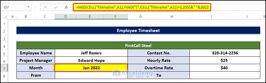
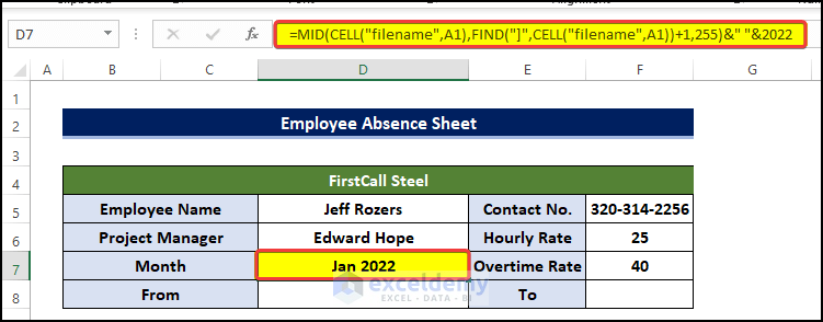
- Select cell D7 and enter the following formula:
=MID(CELL("filename",A1),FIND("]",CELL("filename",A1))+1,255)&" "&2022
Formula Breakdown
This formula returns the sheet name in the selected cell.
- CELL(“filename”,A1): The CELL function gets the complete name of the worksheet
- FIND(“]”,CELL(“filename”,A1)) +1: The FIND function will give you the position of ] and we’ve added 1 because we require the position of the first character in the name of the sheet.
- 255: Excel’s maximum word count for the sheet name.
- MID: The MID function uses the text’s position from start to end to extract a specific substring.
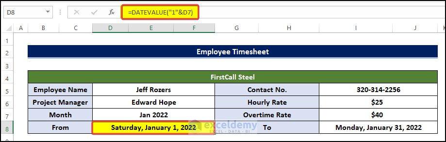
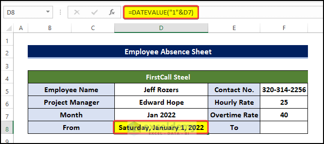
- After then, select the cell D8 and enter the following formula:
=DATEVALUE("1"&D7)
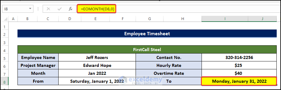
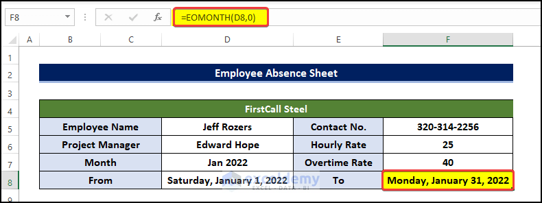
- Then select cell I8 and enter the following formula
=EOMONTH(D8,0)
- This cell value will depend upon the name of the sheet.
- For example, the sheet name here is Jan, so we are seeing the Month name stated in the D7 cell.
- We can make multiple sheet names after different months and the formula of these cells will update automatically.
Step 3: Formulize Daily Input Table
In the input table, dates and days will be dynamic depending on the value of the sheet title. It will make the sheet more vibrant and smoother. The TEXT and IF functions are going to be used here.
- Then, in cells in the B10:J10 range, construct headings like Date, Day, and In time, etc.
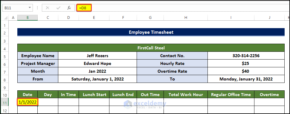
- Select cell B11 and enter the following formula:
=D8
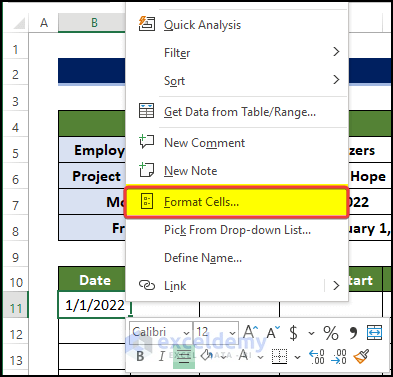
- Then right-click on the cell and from the context menu, click on the Format Cells.
In the format cell window, click on the Number and then click on Custom.
- In the custom option, type “d” in the Type field.
- And then press OK.
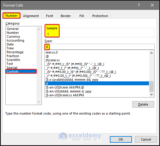
- After this, we can see that the date in cell B11 is now set to the numerical serial.
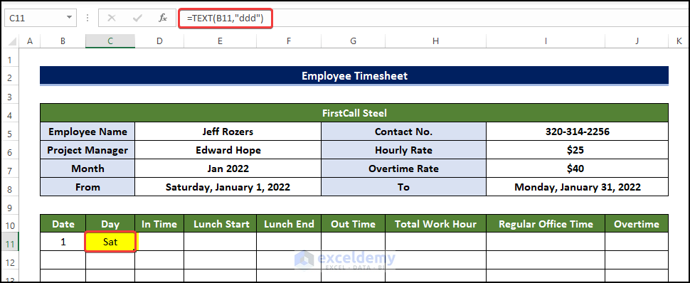
- Select cell C11 and enter the following formula:
=TEXT(B11,"ddd")
- This formula will show the day of the date shown in cell C11.
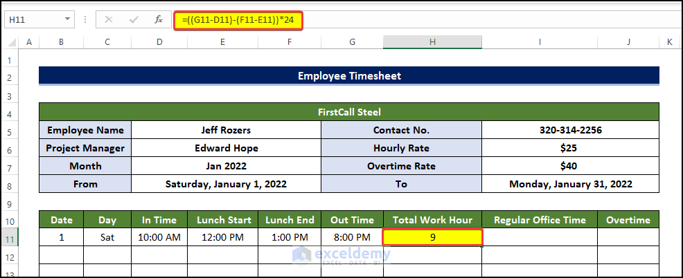
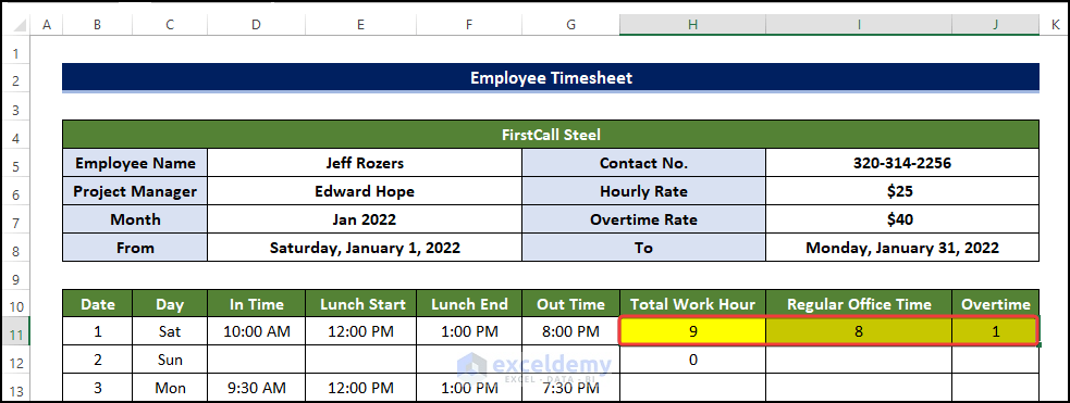
- Then select cell H11 and enter the following formula:
=((G11-D11)-(F11-E11))*24
This formula will calculate the Total Work Hour in the office.
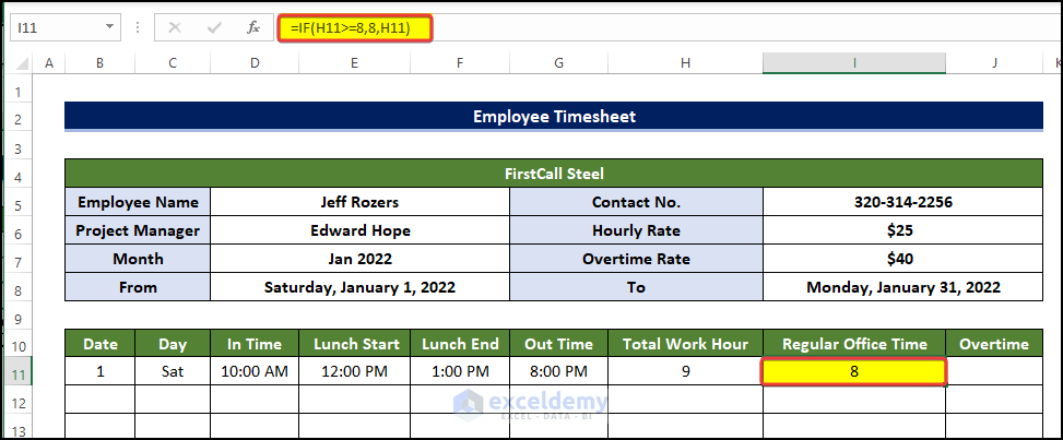
- After this, select cell I8 and enter the following formula:
=IF(H11>=8,8,H11)
This formula will place the Regular Office Time in the I11 cell if the total work hour is greater than 8.
Formula Breakdown
- IF(H11>=8,8,H11): checks whether a condition is met and returns one value if TRUE and another value if FALSE. Here, H11>=8 is the logical_test argument that compares the value in the H11 cell with 8. If this value is greater than or equal to 8 then the function returns 8 (value_if_true argument) otherwise it returns the value of the cell H11 (value_if_false argument).
- Output: 9
- Then we calculate the overtime by subtracting the Regular Office Time from the Total Work Hour.
- Select cell J11 and enter the following formula
=IF(H11<=8,0,H11-I11)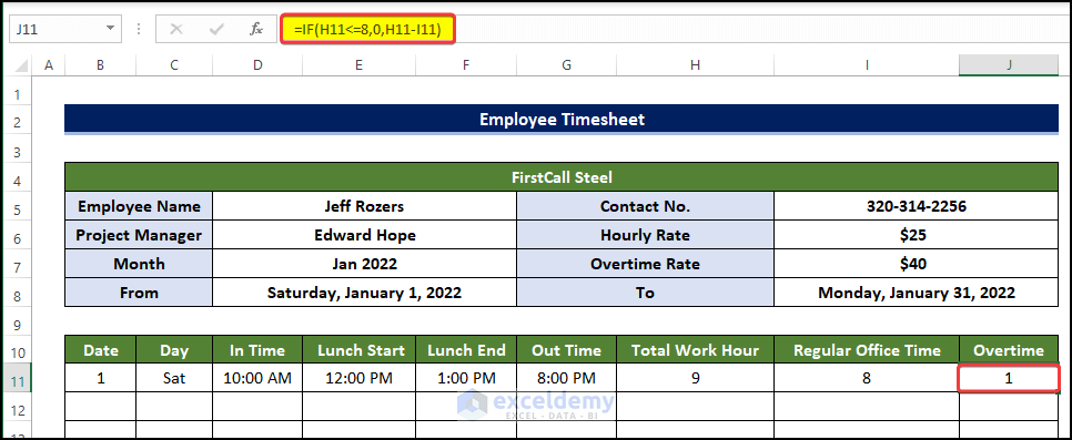
Formula Breakdown
- IF(H11<=8,0,H11-I11) : checks whether a condition is met and returns one value if TRUE and another value if FALSE. Here, H11<=8 is the logical_test argument that compares the value in the H11 cell with 8. If this value is less than or equal to 8 then the function returns 0 (value_if_true argument) otherwise it returns the value H11-I11 (value_if_false argument).
- Output : 1
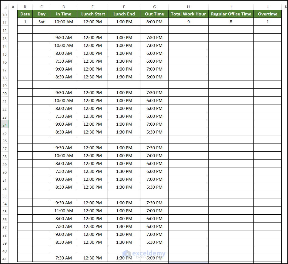
Step 4: Fill Up Input Table with Information
As we have the first-row information, we can now fill the rest of the sheet with entry data. Creating an employee timesheet in Excel is a must.
We enter entry data from the starting date of the month to the end of the month. The blank rows represent the Sunday where there are no data because Sunday is actually a holiday. Other values will be calculated in the subsequent step.
Step 5: Further Formulize of Table
- Now we have the data entry for each day, but we still don’t have each day of the month. Yet, To have each day and date we will use the following functions TEXT, and IF.
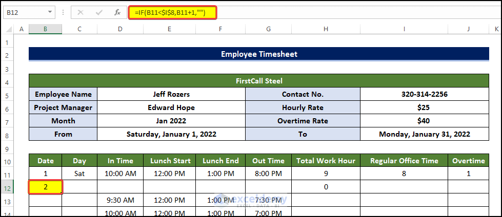
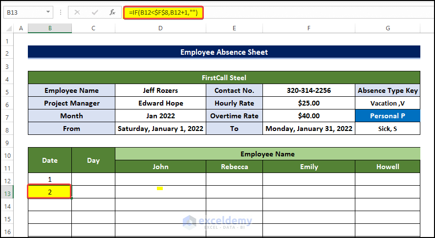
we need to enter the following formula in the cell B12:
=IF(B11<$I$8,B11+1,"")
- Here, B11 and I8 represent the first date of the month and the last date of the month successively. Then the formula returns the next date of the date in cell B11. Otherwise, it will show nothing.
- Click OK after this.
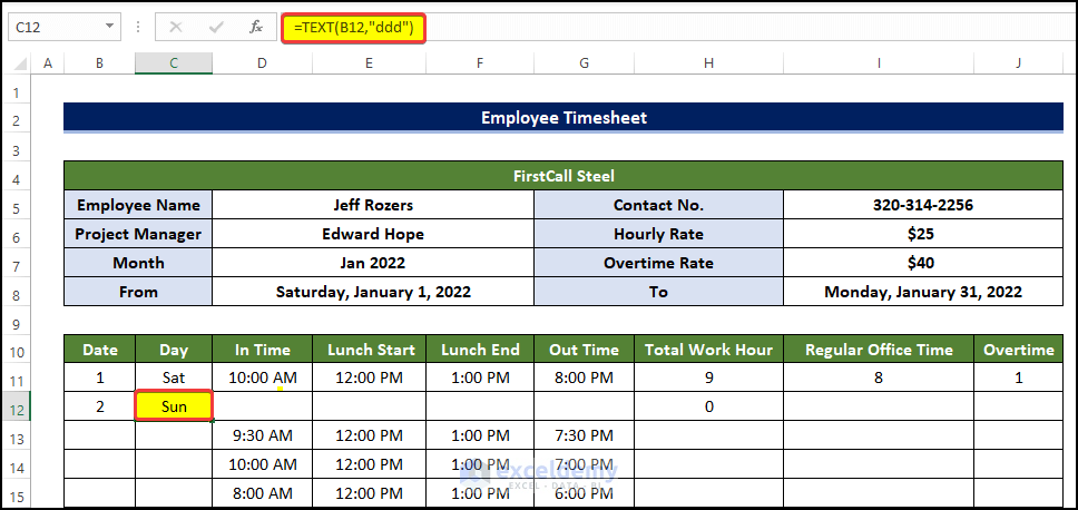
- Select cell C12.
- Enter the following formula:
=TEXT(B12,"ddd")
- This formula will extract the Day of the Date in cell B12.
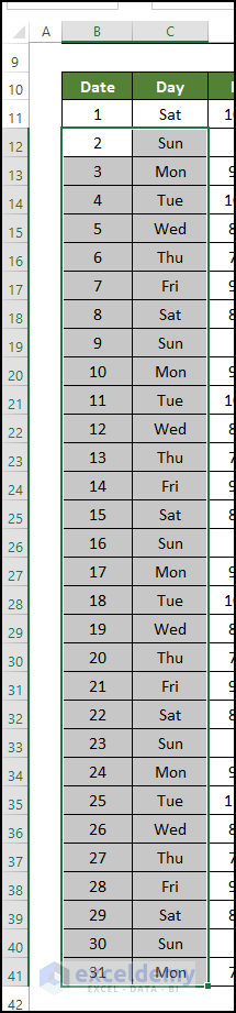
- We need to fill in the Date and Day for the month.
- To do this, select the range of cell B12:C12
- Then select the Fill Handle and drag it to cell C41.
- Doing this will fill the range of cells B12:C41 with the dates and their corresponding days.
- Now it’s time to fill the Total Work Hour with Regular Office Time and Overtime.
- Select the range of cell H11:J11.
- Then drag the Fill Handle to cell J42.
Step 6: Use Conditional Formatting to Highlight Weekends
To create an employee timesheet in Excel, we must include weekends. As Sunday is the weekly holiday, we don’t have to input anything into those cells. We will highlight those cells with Conditional Formatting. Let us go through the steps.
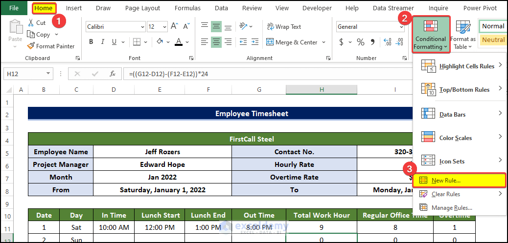
- select cell D11, and move to the Home tab.
- Click on the Conditional Formatting drop-down on the Styles group.
- select New Rule from the available options.
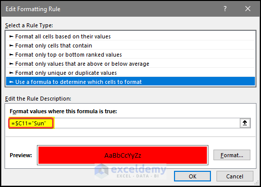
- Suddenly, it opens the New Formatting Rule wizard.
- choose to Use a formula to determine which cells to format under the Select a Rule Type section.
- Then, we’ve to make some edits in the Edit the Rule Description section.
- Later, write down =$C11=”Sun” in the Format values where this formula is true box.
- Then choose the red cell fill color from the Format option.
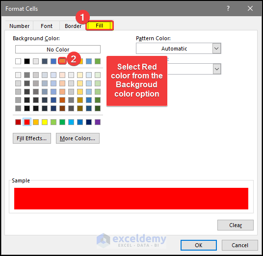
- After clicking Format, we will be taken to a new window.
- In that window, we first move to the Fill and tab.
- Choose the Red color from the available options.
- Click OK.
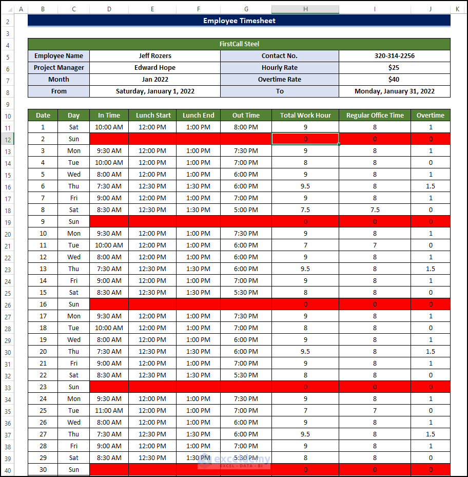
- After that, we will be taken to the Conditional Formatting Rules Manager.
- Click OK after this.
- Then we can observe that Sundays are now marked with a red color.
Step 7: Estimate Final Payment
As our Sundays and the other entry information are now filled up, we can calculate the total income based on the total hours and the overtime periods. The SUM function is going to be used here.
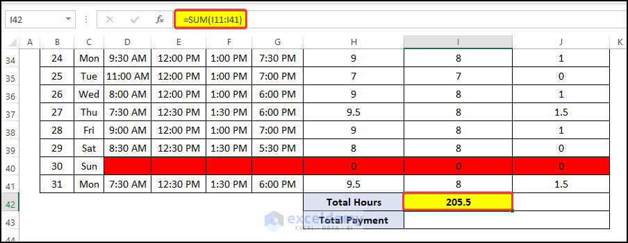
- To begin with, go to cell H11.
- the following formula:
=SUM(I11:I41)
Here we calculated the Total Hours worked by that particular employee.
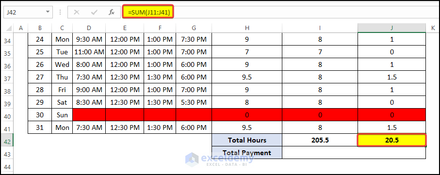
- Then we select cell J42 and enter the following formula:
=SUM(J11:J41)
We calculated the overtime worked by that specific employee.
- Finally, we are going to calculate the Total Payment of that employee.
- Select cell I43 and enter the following formula:
=I42*I6+J42*I7
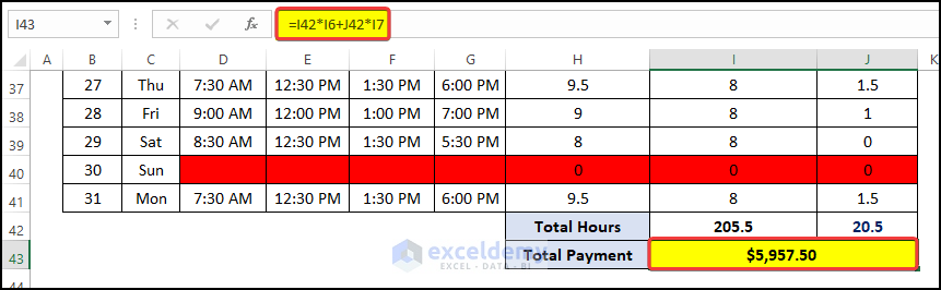
And this is how we managed to create an employee Timesheet in Excel.
How to Create Employee Absence Schedule in Excel
Here we are going to create an absence schedule in Excel using various formulas, These formulas will make the sheet more dynamic and automatic.
Step 1: Prepare Basic Information Structure
Here, we’re showing the full process in different steps so that it is easy to understand. To make it easier to understand, we break down the entire process into its component parts here.
First of all, we need to create a basic outline of the monthly worksheet. So, just follow along.
- In cell B4, write down the name of the company. Here, we assumed it FirstCall Steel.
- Also, place the Employee Name, Project Manager’s name, Contact No, Hourly Rate, and Overtime Rate.
Step 2: Formalize Basic Information Employee Absence Schedule
In the next step, we will formalize the information to make it more dynamic and user-friendly. The functions used here are MID, CELL, FIND, DATEVALUE, and EOMONTH.
- Select cell D7 and enter the following formula:
=MID(CELL("filename",A1),FIND("]",CELL("filename",A1))+1,255)&" "&2022
Formula Breakdown
This formula returns the sheet name in the selected cell.
- CELL(“filename”,A1): The CELL function gets the complete name of the worksheet
- FIND(“]”,CELL(“filename”,A1)) +1: The FIND function will give you the position of and we’ve added 1 because we require the position of the first character in the name of the sheet.
- 255: Excel’s maximum word count for the sheet name.
- MID: The MID function uses the text’s position from start to end to extract a specific substring.
- Select cell D8 and enter the following formula:
=DATEVALUE("1"&D7)
- Select cell E8 and enter the following formula:
=EOMONTH(D8,0)
- Now we are going to color-code the cells based on the input values in the entry data.
- We will put any kind of Vacation as V, Sick Leave as S, and Personal Leave as P.

Step 3: Formulize Daily Input Table
In the input table, dates and days will be dynamic depending on the value of the sheet title. It will make the sheet more vibrant and smoother. The IF and TEXT functions are going to be used here.
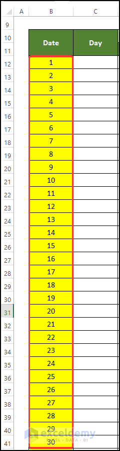
- Select cell B12 and enter the following formula:
=D8
- While selecting the cell, right-click on the mouse. From the context menu, click on the Format Cells.
- In the format cell window, click on the Number and then click on Custom.
- In the custom option, type “d” in the Type field.
- And then press OK.
- Select cell B13 and enter the following formula:
=IF(B12<$I$8,B12+1,"")
- Here, B12 and I8 represent the first date of the month and the last date of the month successively. Then the formula returns the next date of the date in cell B12. Otherwise, it will show nothing.
- Click OK after this.
- Then drag the Fill Handle to cell B41.
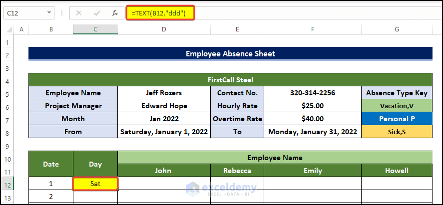
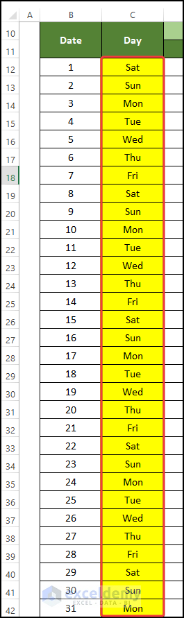
- Select cell C12 and enter the following formula:
=TEXT(B12,"ddd")This formula will show the day of the date shown in cell C12.
- Then drag the Fill Handle to cell B41.
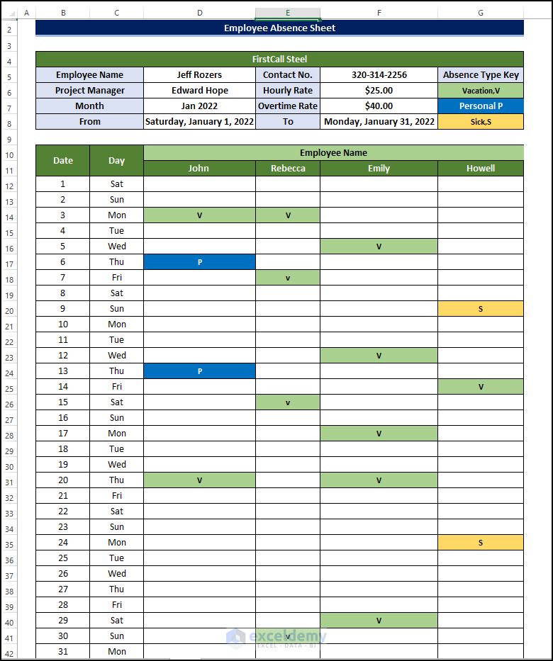
Step 4: Input and Color Code Information
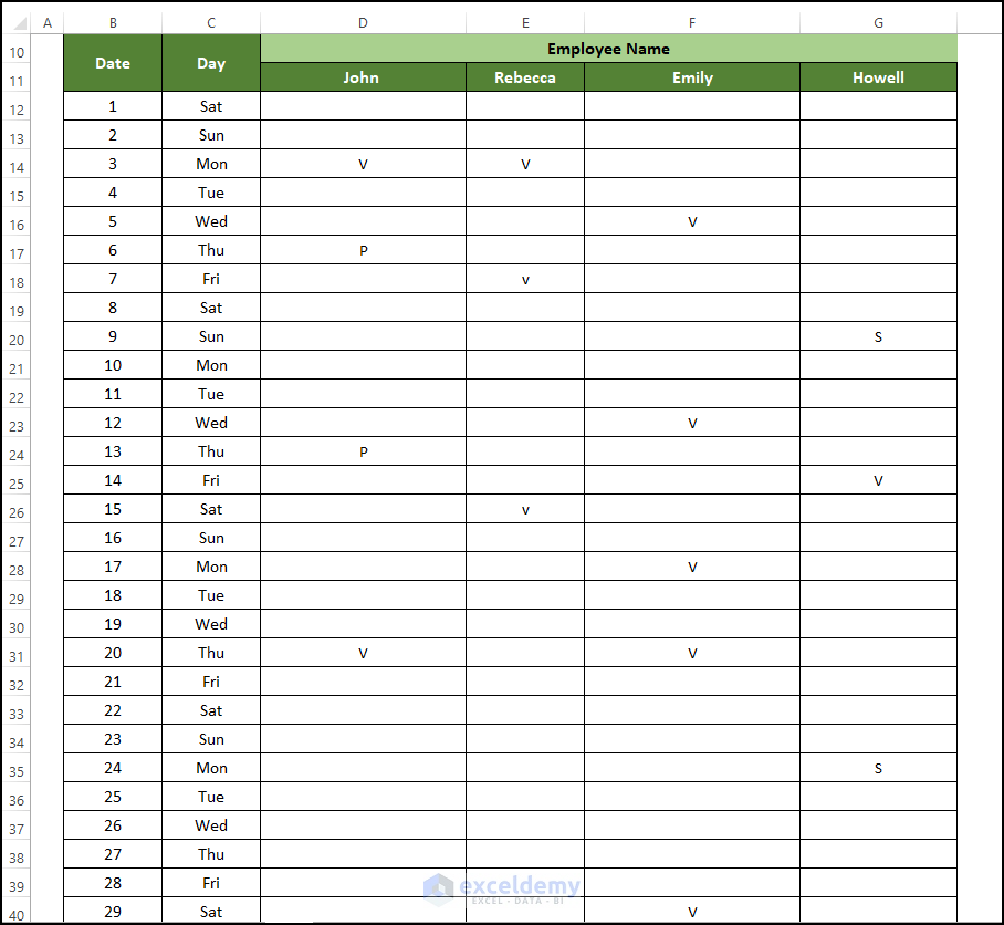
We enter vacation type depending on data from the starting date of the month to the end of the month. The blank rows represent the Sundays where there is no data because those dates are holidays anyway.
We fill up the table with the vacation date with color coding as shown at the beginning of the chart.
- After we fill up the table with the vacation code, we can color them using Conditional Formatting.
- For this, go to the Home tab > Conditional Formatting > New Rules.
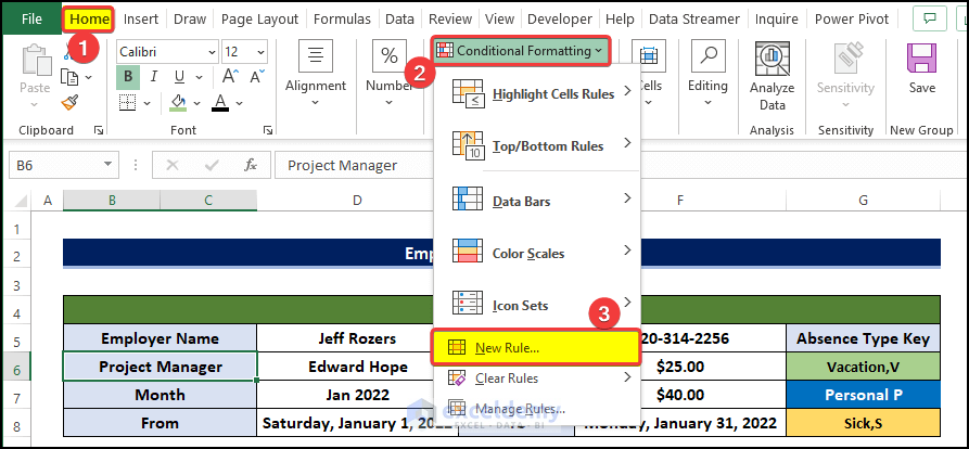
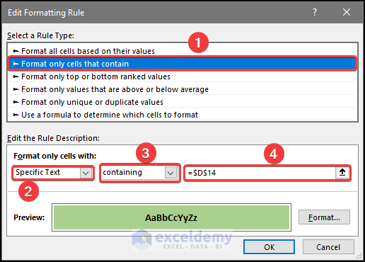
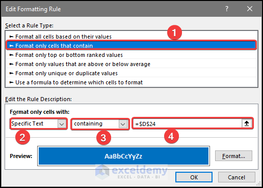
- Then in the Edit Formatting Rule, Select Format only cells that contain in the Select a Rule Type option.
- Then select Specific Text in the first drop-down from the left side.
- Select Containing from the Second drop-down from the left
- Then select $D$14 in the third drop-down from the left side.
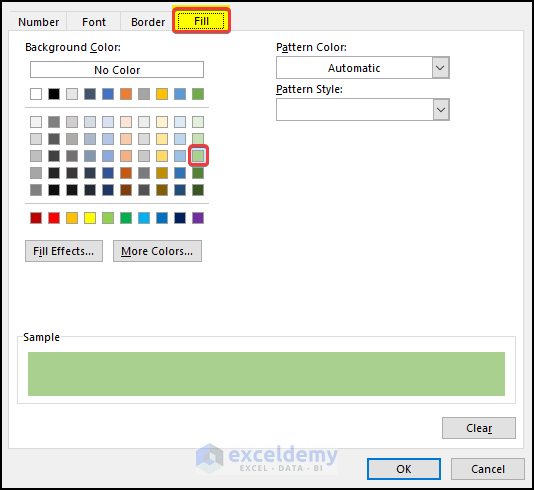
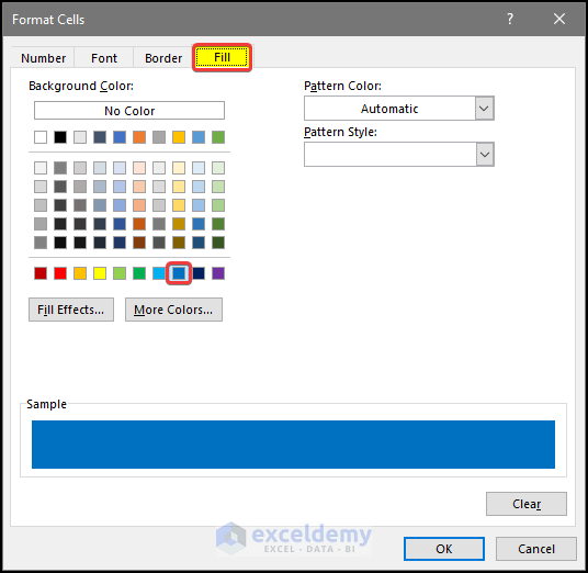
- Click Format after this.
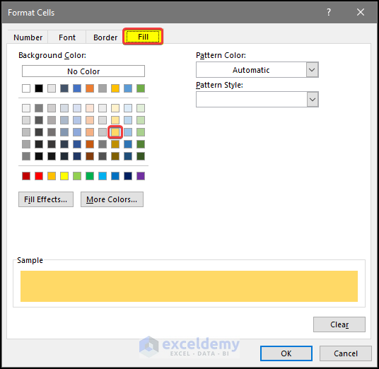
- In the Format window, go to the Fill tab, and then pick the color of your choice.
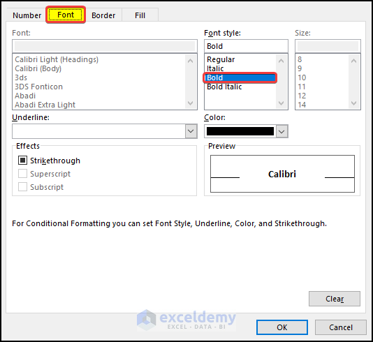
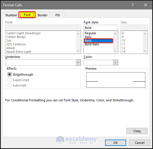
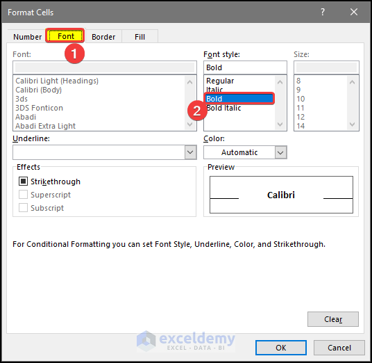
- Then switch back to the Font tab and make the font Bold in the Font style option.
- Click OK after this.
- Again switch back to the Conditional Formatting.
- Then in the Edit Formatting Rule.
- Select Format only cells that contain in the Select a Rule Type option.
- Then select Specific Text in the first drop-down from the left side.
- Select Containing from the Second drop-down from the left
- Then select $D$14 in the third drop-down from the left side.
- Click Format after this.
- In the Format window, go to the Fill tab, and then pick the color of your choice.
- Then switch back to the Font tab and make the font Bold in the Font style option.
- Click OK after this.
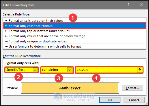
- Then in the Edit Formatting Rule.
- Select Format only cells that contain in the Select a Rule Type
- Then select Specific Text in the first drop-down from the left side.
- Select Containing from the Second drop-down from the left
- Then select $D$14 in the third drop-down from the left side.
- Click Format after this.
- In the Format window, go to the Fill tab, and then pick the color of your choice.
- Then switch back to the Font tab and make the font Bold in the Font style option.
- Click OK after this.
- After that we can see that the vacation input table is now filled with the vacations with the color code.
Step 5: Estimate Final Payment
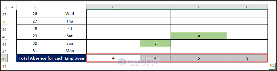
We now calculate the gross vacation taken by the employee by using the COUNTA function.
- Select cell D43 and enter the following formula:
=COUNTA(D12:D42)
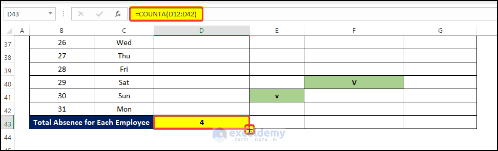
- Then drag the Fill Handle horizontally in the corner of the cell to the cell G43.
And this is how we managed to create an employee absence Timesheet in Excel.
Download Practice Workbook
Download this practice workbook below.
Conclusion
To sum it up, the issue of how we can create an employee Timesheet in Excel in 5 different steps. For this problem, a macro-enabled workbook is available to download where you can practice these methods. And, Feel free to ask any questions or feedback through the comment section.
<< Go Back to Timesheet | Formula List | Learn Excel
Get FREE Advanced Excel Exercises with Solutions!
