This article describes the way of creating timesheets for an individual employee, all employees counting lunch break and overtime with final payment. More importantly, this article shows another example of making a timesheet considering working days only excluding holidays, weekends, and taken leaves.
In workplaces, the Timesheet is a trendy term. It is a method that is used to record employee time records in the office. Originally, this method was developed to calculate salary at the end of each month, considering overtime hours and break or lunch hours. Microsoft Excel has made our work easier to create a timesheet.
In this article, we will create a timesheet in Excel with 3 useful examples.

How to Create a Timesheet in Excel: 3 Useful Examples
To describe the method of creating a timesheet, we will demonstrate here 2 useful examples for better understanding. Let’s follow the procedure below.
Example 1: Create a Timesheet in Excel for Individual Employee
In this example, we will make a timesheet of a single employee in a company. Also, we will calculate the payment at the end. Follow the steps carefully.
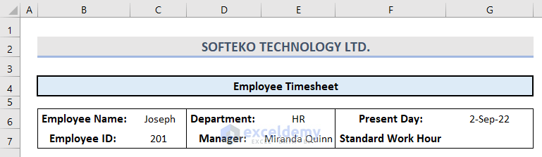
- First, insert the company name, page title, and other information (see image below) in rows 2, 3, 6, and 7 respectively.
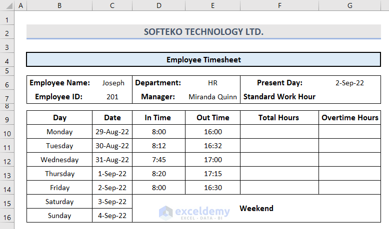
- Then, create a table with the titles Day, Date, In Time, Out Time, Total Hours, and Overtime Hours.
- Afterward, insert information into the respective titled cells like this:
- Following, go to the Home tab and select Fill Color under the Font group.
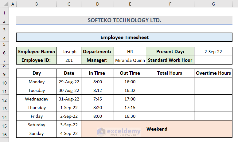
- From here, customize your table with your preferred colors and the final output looks like this:
- Now, insert this formula in cell F10.
=E10-D10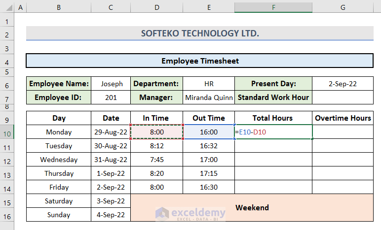
- Then, press Enter.
- Here, you will see the Total Hours of the job done on Monday.
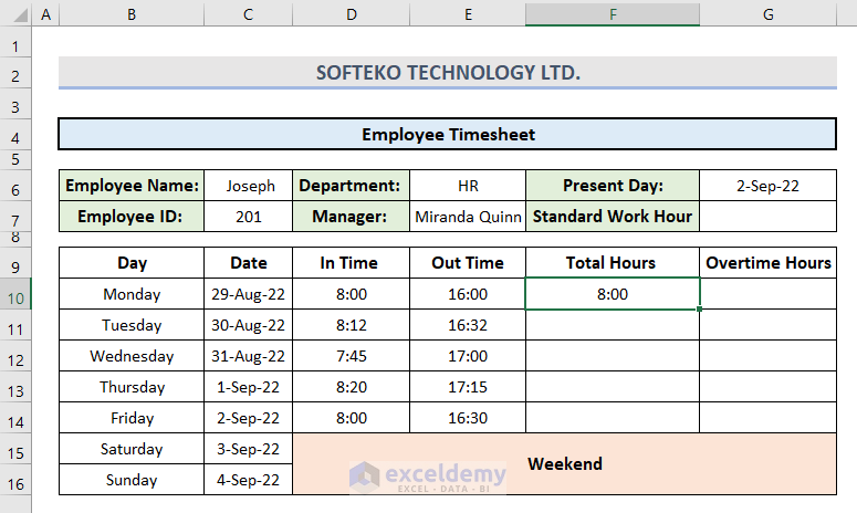
- Then, use the AutoFill tool to get the result for the whole week.

- Next, insert this formula in cell G7 to calculate the Standard Work Hour using the TIME function.
=TIME(8,0,0)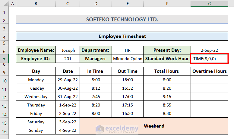
- Now, insert this formula in cell G10.
=IF(F10>G7,(F10-$G$7),0)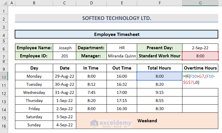
- Following, drag the bottom corner of cell G10 up to cell G14 to calculate the Overtime Hours of each day.
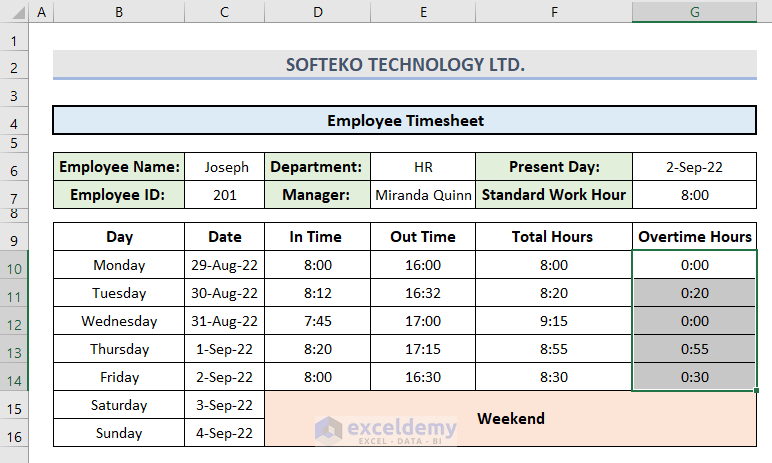
Here, we applied the IF function to determine a logical comparison between Total Hours and Standard Work Hour.
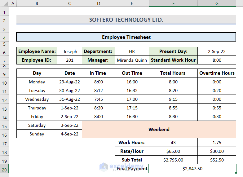
- So far, we have successfully created a timesheet in Excel for an individual employee.
- Along with it, let us calculate the Final Payment based on Work Hours and Rate/Hour.
- Initially, insert this formula in cell F17 to calculate the Work Hours of a week.
=SUM(F10:F14)*24
- Similarly, count total Overtime Hours with this formula in cell G17.
=SUM(G10:G14)*24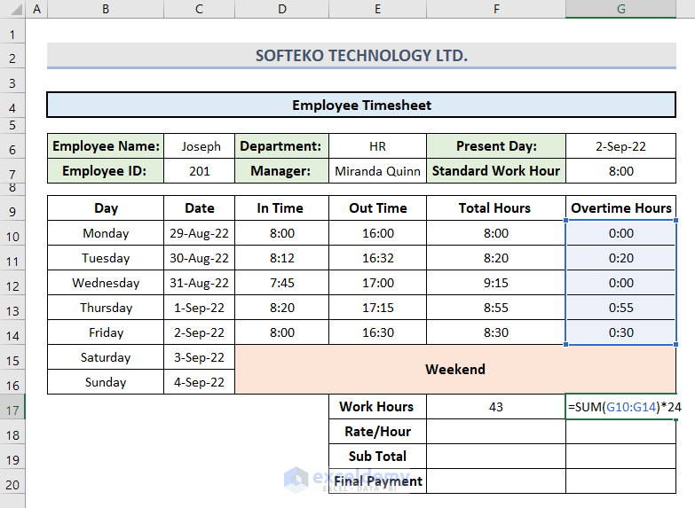
Here, we used the SUM function to count the total hours in selected cells. Along with it, we multiplied it by 24 to get the result in 24-hour format.
- Next, insert this formula in cell F19 to calculate Sub Total based on Rate/Hour.
=F17*F18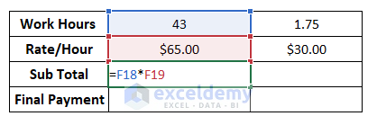
- Similarly, count it for Overtime Hours with this formula.
=G17*G18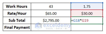
- Lastly, apply this formula to find the Final Payment in cell F20.
=F19+G19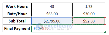
- Finally, press Enter, and you will get your final output.
Example 2: Make an Excel Timesheet Template for All Employees
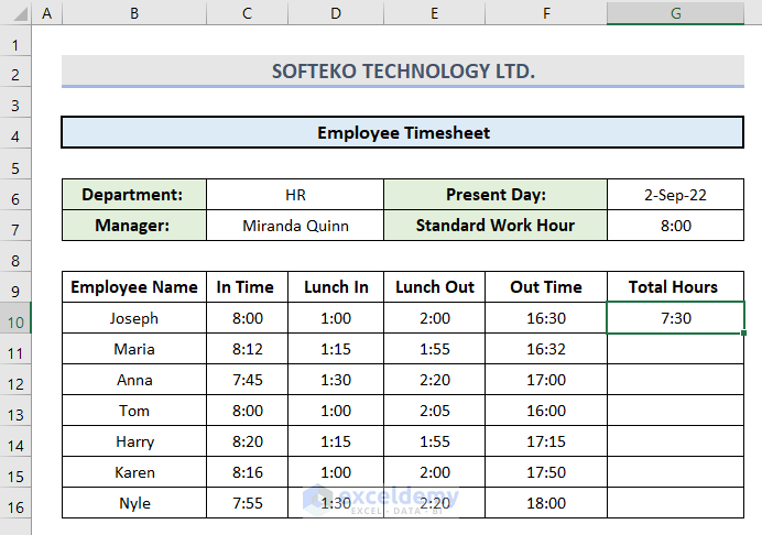
In this second one, we will create an Excel timesheet for all employees in the department. We will also include the lunch hours this time. Let’s see how it works.
- In the beginning, insert all the information in your worksheet as per the image below:
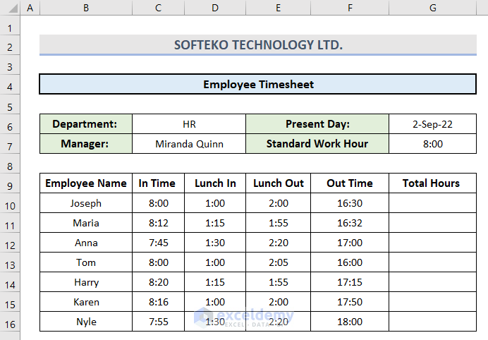
- Make sure to insert the Standard Work Hour as described in the 1st example.
- Now, insert this formula in cell G10.
=(F10-E10)+(D10-C10)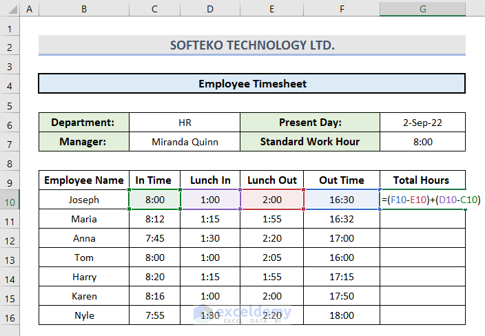
- Afterward, press Enter.
- Here, you will see the first input of the Total Hours of Joseph.
- Lastly, use the Fill Handle tool to get a similar output for all the employees in cell range G11:G16.
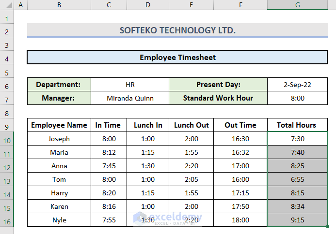
- That’s it, we have our timesheet template in Excel.
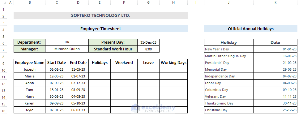
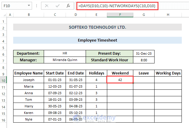
Example 3: Create an Excel Timesheet Template Counting Working Days (Excluding Holidays, Weekends, & Taken Leaves)
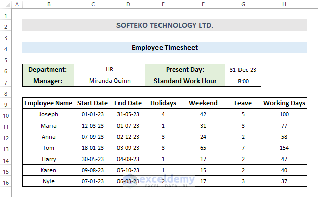
- First, here is a timesheet to calculate the total working days of some employees.
- Now, insert the following formula in cell E10.
=SUMPRODUCT(($K$7:$K$16>=C10)*($K$7:$K$16<=D10))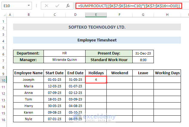
Formula Breakdown Formula Breakdown
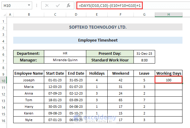
The above formula calculates the number of days between two dates (D10 and C10), while subtracting the specified number of days in cells E10, F10, and G10. The “+1” at the end is added to include the starting day in the count. 1. What is the formula for timesheet in Excel? The formula for calculating total hours in a timesheet in Excel is typically “=SUM([Range of Hours])”. 2. How do I get AM PM in Excel? We can use the time format code “h:mm AM/PM” or “h:mm am/pm” in the cell formatting options. 3. How do I create a 1 hour interval in Excel? You can use the formula “=A1 + TIME(1,0,0)” to create a 1-hour interval in Excel. Get this template to practice by yourself. Finally, we are concluding this article. Hope it was a helpful one for you on how to create a timesheet in Excel with 3 useful examples. Let us know your suggestions in the comment section. Have a nice day! << Go Back to Timesheet | Formula List | Learn Excel
=DAYS(D10,C10)-NETWORKDAYS(C10,D10)
=DAYS(D10,C10)-(E10+F10+G10)+1
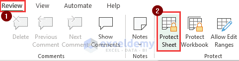
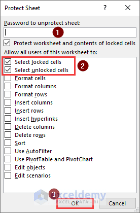
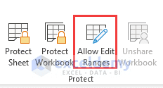
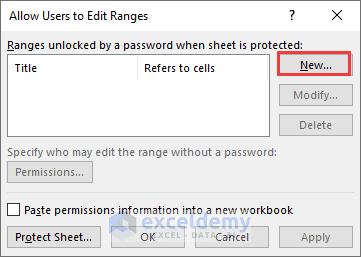
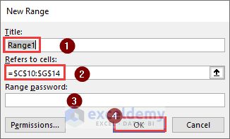
How to Protect Timesheet in Excel
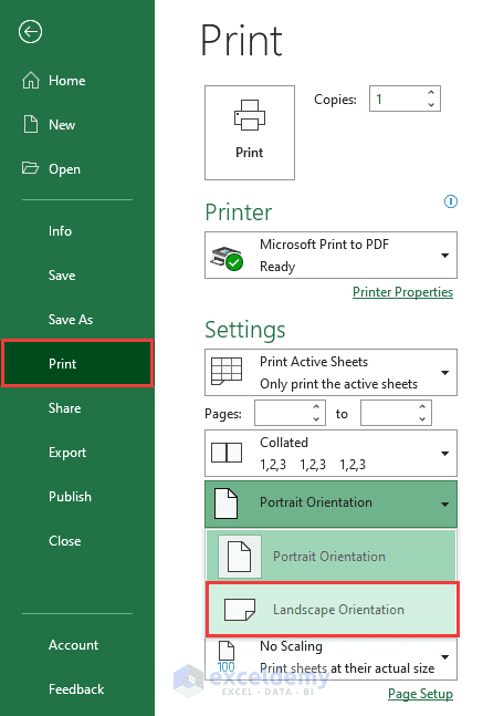
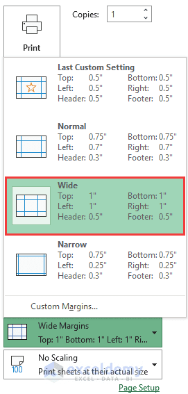
How to Print Timesheet in Excel
Things to Remember
Frequently Asked Questions
Conclusion

