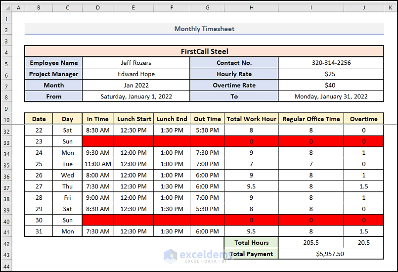
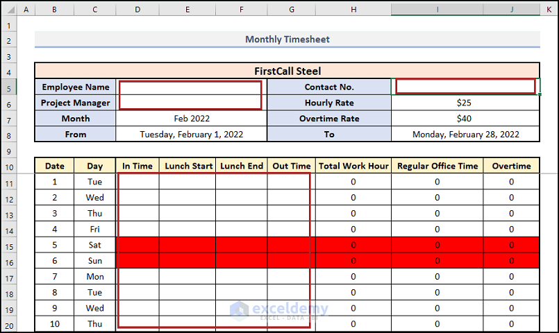
We’ll use a sample dataset from a fictional HR’s information for an employee. Here’s the overview of the timesheet we’ll make.
Step 1- Create a Basic Outline of the Monthly Timesheet in Excel
- Construct a heading in cell B2 and put it the Heading 2 cell style. We named it Monthly Timesheet.
- In cell B4, write down the name of the company.
- Place the Employee Name, Project Manager’s name, Contact No., Hourly Rate, and Overtime Rate. Create empty cells for Month, From, and To values.
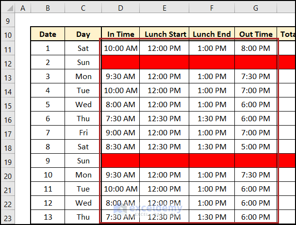
- In cells in the B10:J10 range, construct some headings like Date, Day, In time, etc.

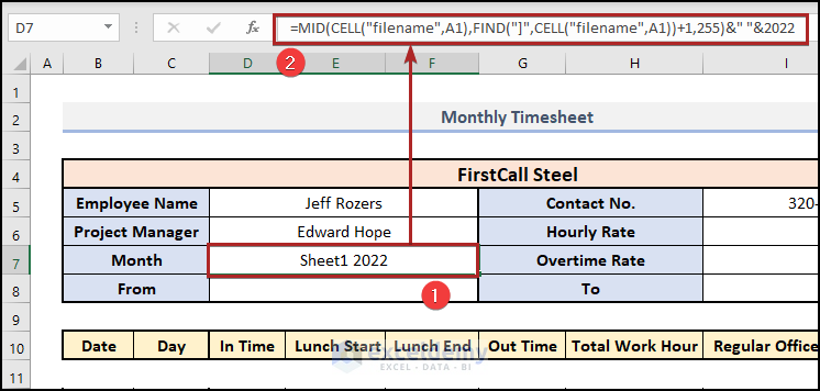
- Select cell D7 (Month).
- Use the formula below in it:
=MID(CELL("filename",A1),FIND("]",CELL("filename",A1))+1,255)&" "&2022
Formula Breakdown
This formula returns the sheet name in the selected cell.
- CELL(“filename”,A1): The CELL function gets the complete name of the worksheet
- FIND(“]”,CELL(“filename”,A1)) +1: The FIND function will give you the position of ] and we’ve added 1 because we require the position of the first character in the name of the sheet.
- 255: Excel’s maximum word count for the sheet name.
- MID: The MID function uses the text’s position from start to end to extract a specific substring.
- Press the Enter key.
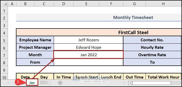
- You’ll get the sheet name and the manually input year 2022.
- Change the name of the sheet to Jan.
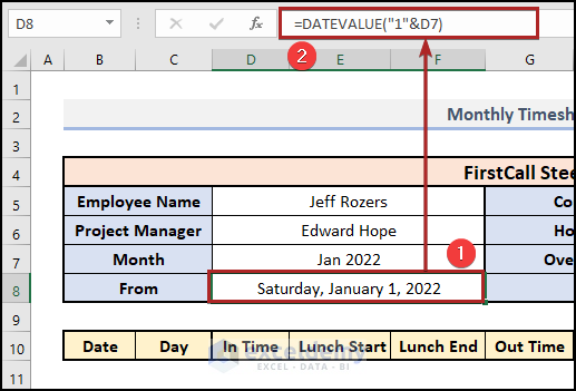
- Select cell D8.
- Input the following formula.
=DATEVALUE("1"&D7)
Here, D7 represents the month of Jan 2022. A date that is stored as text can be changed into a serial number that Excel can identify as a date using the DATEVALUE function.
- Hit Enter.
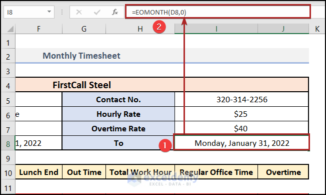
- Select cell I8 to show the ending date of that month.
- Use the following formula in the cell and press Enter.
=EOMONTH(D8,0)
The EOMONTH function is used to determine the end of the month.
Step 2 – Generate the Dates and Corresponding Days
- Select cell B11.
- Paste in the following formula and press the Enter key.
=D8
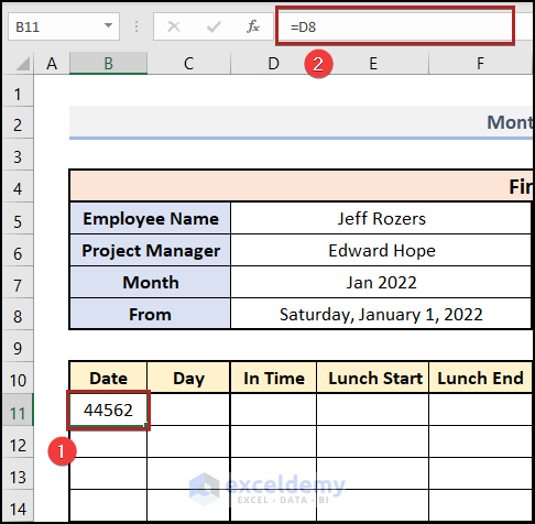
The date is shown in the General Number format. We’ll need to convert it.
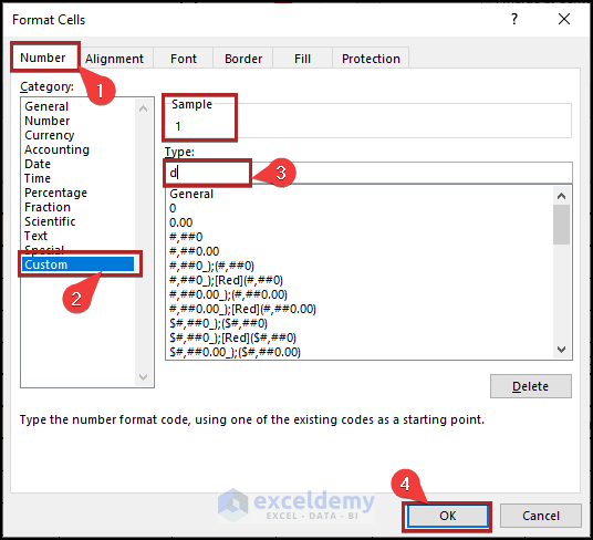
- Press Ctrl + 1. This opens the Format Cells dialog box.
- Go to the Number tab.
- Select Custom from the Category section.
- In the Type box, write d.
- Click OK.
- You’ll get the date of the first day of the month, displaying only the date part.
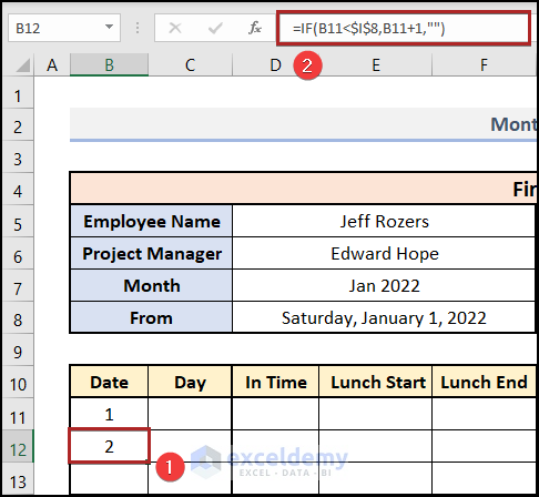
- Select cell B12.
- Paste the following formula into the cell.
=IF(B11<$I$8,B11+1,"")
- Hit Enter.
- Hover over the bottom-right corner of cell B12. The cursor will change to a plus (+) sign. It’s the Fill Handle tool.
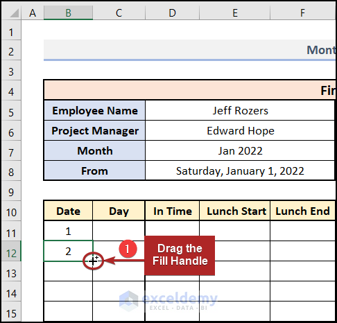
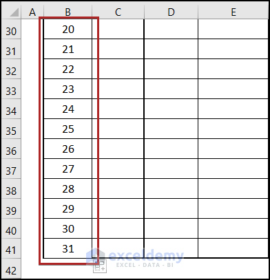
- Use the Fill Handle tool and drag it to cell B41 to show the other days of the month.
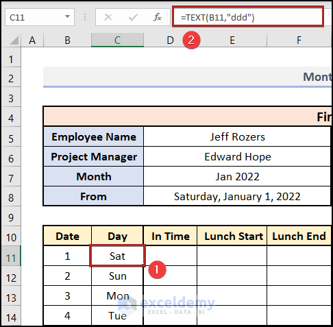
- Select cell C11.
- Put the following formula into the Formula Bar.
=TEXT(B11,"ddd")
ddd shows the first three letters of the weekday.
- Press Enter.
Step 3 – Specify the Weekends
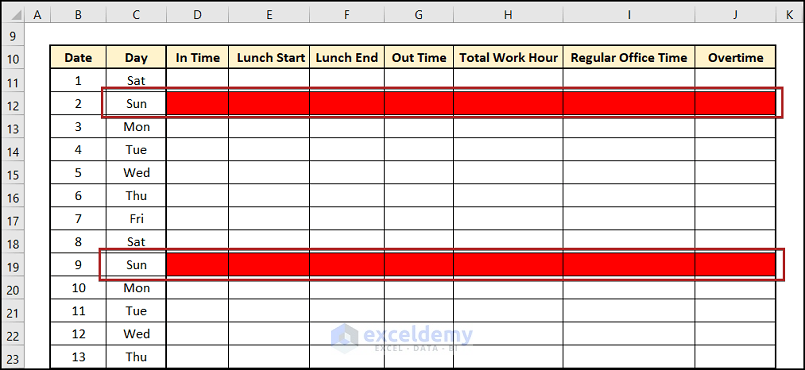
We’ll consider the Sunday as the weekend and will highlight those cells with Conditional Formatting.
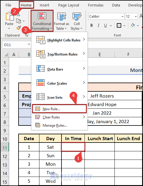
- Select cell D11.
- Move to the Home tab.
- Click on the Conditional Formatting drop-down on the Styles group.
- Select New Rule from the available options.
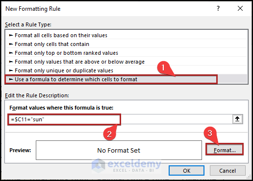
- This opens the New Formatting Rule wizard.
- Choose Use a formula to determine which cells to format under the Select a Rule Type section.
- Insert =$C11=”Sun” in the Format values where this formula is true: box.
- Select the Format button.
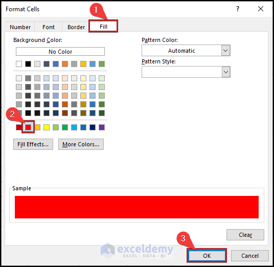
- The Format Cells wizard opens.
- Move to the Fill tab.
- Choose the Red color from the available options.
- Cick OK.
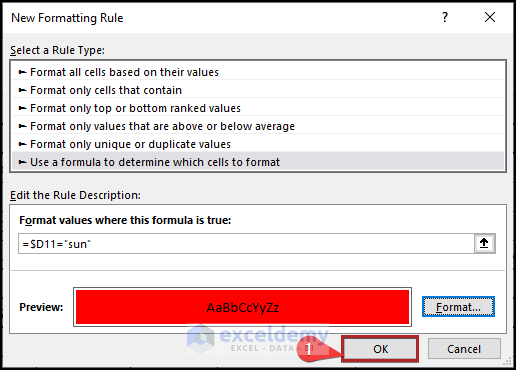
- This returns us to the New Formatting Rule dialog box.
- Click OK again.
- Use the Fill Handle tool to expand the formatting across the D11:J41 range.
Step 4 – Enter Data
- Enter the necessary data like In Time, Lunch Start, Lunch End, and Out Time in the sheet. We’ve put some sample data into the sheet.
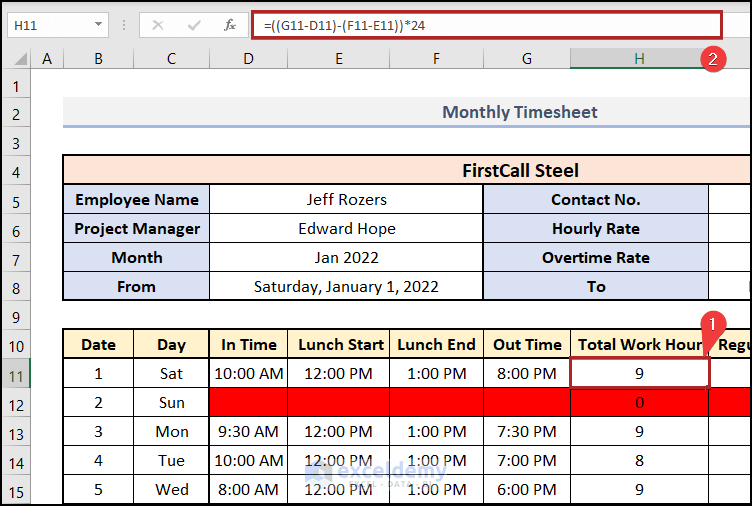
Step 5 – Calculate the Total Work Hours
- Go to cell H11 (or wherever you’ve put the value for total work hours for the day).
- Use the following formula.
=((G11-D11)-(F11-E11))*24
The D11 and G11 cells represent the In Time and Out Time while the E11 and F11 cells refer to the Lunch Start and Lunch End time, respectively. The multiplication by 24 converts the time to hours.
- Hit Enter and AutoFill through the column.
Step 5 – Determine Regular and Overtime Hours
We’ll assume anything over 8 working hours (not including the lunch break) is paid overtime.
- Select cell I11.
- Use the following formula.
=IF(H11>=8,8,H11)
The H11 cell refers to the Total Work Hours.
Formula Breakdown
- IF(H11>=8,8,H11) → checks whether a condition is met and returns one value if TRUE and another value if FALSE. Here, H11>=8 is the logical_test argument that compares the value in the H11 cell with 8. If this value is greater than or equal to 8 then the function returns 8 (value_if_true argument) otherwise it returns the value of the cell H11 (value_if_false argument).
- Output → 9
- Hit Enter.
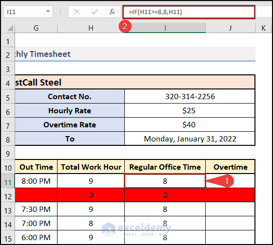
Note: Here, we’ve considered 8 hrs as the regular working time.
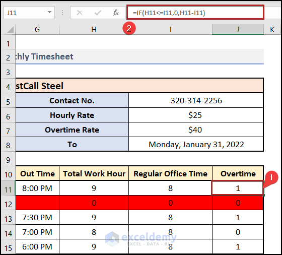
- Select cell J11 and put the following formula into the cell.
=IF(H11<=8,0,H11-I11)
Here, the H11 and I11 cells point to the Total Work Hour and Regular Office Time respectively.
Formula Breakdown
- IF(H11<=8,0,H11-I11) → checks whether a condition is met and returns one value if TRUE and another value if FALSE. Here, H11<=8 is the logical_test argument that compares the value in the H11 cell with 8. If this value is less than or equal to 8 then the function returns 0 (value_if_true argument) otherwise it returns the value H11-I11 (value_if_false argument).
- Output → 1
- Hit Enter.
- AutoFill the formulas throughout the columns.
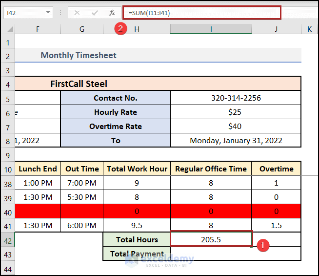
Step 7 – Compute the Total Payment
- Select cell I42.
- Insert the following formula.
=SUM(I11:I41)
- Hit Enter.
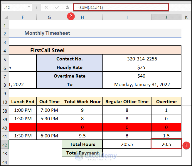
- Go to cell J42.
- Use the formula below.
=SUM(J11:J41)
- Hit Enter.
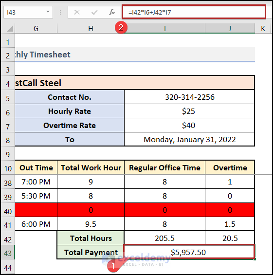
- Select cell I43 and enter the following formula.
=I42*I6+J42*I7
In the above formula, I42, and I6 cells indicate the Total Hours (Regular Office Time) and the Hourly Rate of $25. Additionally, the J42 and I7 cells refer to the Total Hours (Overtime) and the Overtime Rate of $40.
- Hit Enter.
Step 8 – Generate a Timesheet for Another Month
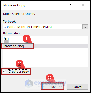
- Right-click on the Sheet Name of the Jan worksheet.
- Select Move or Copy.
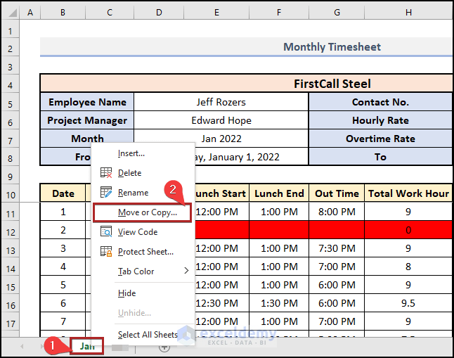
- Select the options as shown in the image below and click on OK.
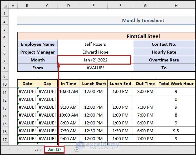
- The cell D7 gets changed with the sheet name.
- The start and end date of the month get changed in cells D8 and I8 automatically.
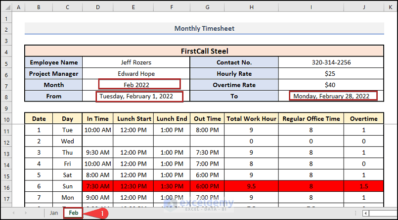
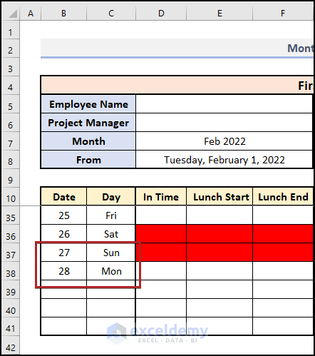
- In this sheet, we’ve assumed 2 weekly holidays: Sat and Sun. You can change this according to your preferences.
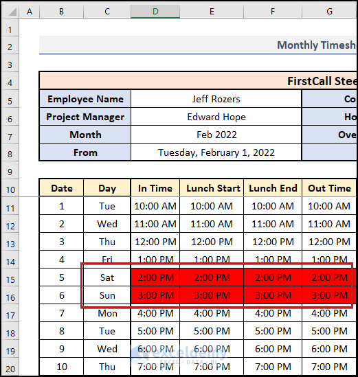
- Clear all previous entries.
- The number of days automatically changed according to the month.
Download the Practice Workbook
<< Go Back to Timesheet | Formula List | Learn Excel
Get FREE Advanced Excel Exercises with Solutions!
