In this article, we will apply timesheet formulas in different time formats that take different kinds of lunch breaks into account.
Example 1 – Timesheet with Fixed Lunch Time
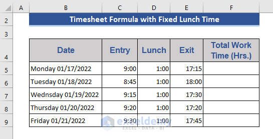
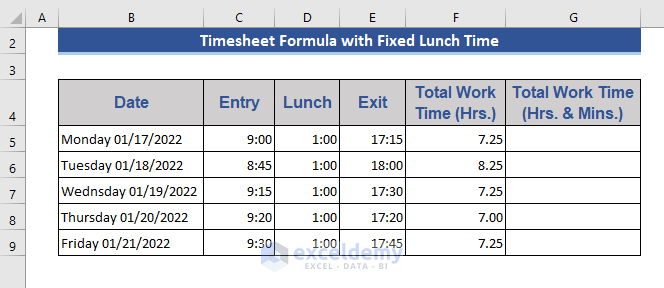
Lunch break procedures vary from one company to another. Here, we assume that the lunch break is fixed at 1:00 pm. We will derive a timesheet formula for this condition using the dataset below, which has columns for the Entry, Exit, and Lunch hours.
Lunch hour is fixed for 1 hour, but the Entry and Exit times vary. Let’s calculate the Total Work Time.
Steps:
- Go to Cell F5.
- Enter the following formula:
=((E5-C5)-D5)*24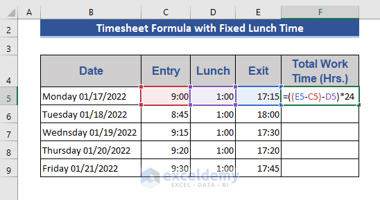
- Press Enter.
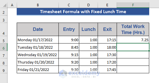
- Drag the Fill Handle icon down to the last cell in the range.
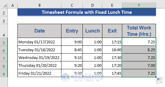
We have the Total Work Hours after subtracting the lunch breaks from the difference between the Entry and Exit times. We’ve represented the effective work time in terms of hours, but we can easily represent the results in terms of hours and minutes too:
- Add a column named Total Work Time (Hrs. & Mins.) to present the work time in the specified format.
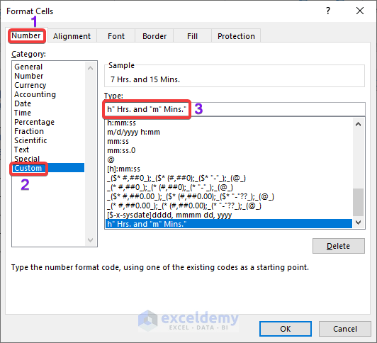
- Select a cell in that column and press Ctrl+1.
The Format Cells window opens.
- Select the Custom category.
- Enter the format as h” Hrs. and “m” Mins.”
- Click OK.
- Enter the below formula in Cell G5:
=(E5-C5)-D5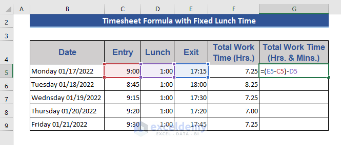
- Press Enter.

- Drag the Fill Handle icon down to the last cell in the range.
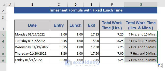
We have the result in Hours and Minutes format.
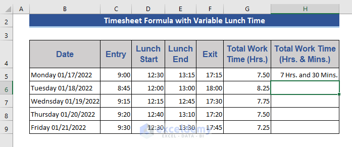
Example 2 – Timesheet with Variable Lunch Break
Now we will consider the case where the lunch break is not fixed. Suppose the employer offers a period of the workday during which employees may take a lunch break for as long as they choose.
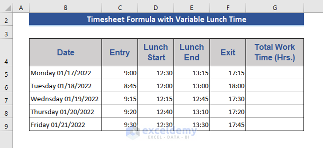
We will consider the above dataset to illustrate this condition, namely that employees can take lunch breaks whenever they want for as long as they want within a specific period.
Steps:
- Go to Cell G5.
- Enter the below formula to subtract the lunch time from the total working time:
=SUM((F5-C5)-(E5-D5))*24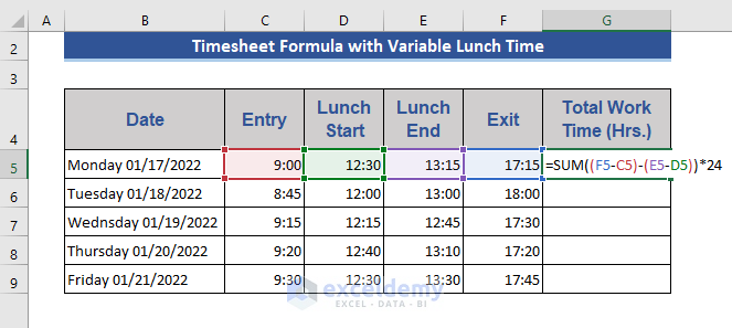
- Press Enter and drag the Fill Handle down to the last cell in the range.
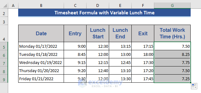
As in the first example, the results are in Hours. To show them in Hours and Minutes form:
- Format the cells as described above.
- In Cell H5 enter the below formula:
=(F5-C5)-(E5-D5)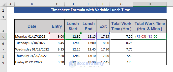
- Press Enter.
- Drag the Fill Handle icon down to the last cell in the range.
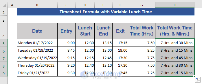
We have the results in Hours and Minutes format.
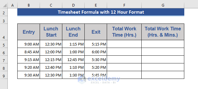
Example 3 – Timesheet with Different Time Formats
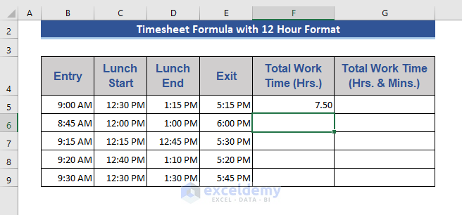
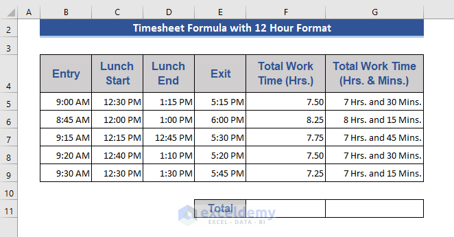
We can apply the 12-hour or 24-hour format to establish the timesheet formula. The above examples were presented in a 24-hour format. Let’s do an example with the 12-hour format using the following dataset, which is in 12-hour format.
Steps:
- In Cell F5, enter the below formula:
=(SUM((C5-B5)+(E5-D5)))*24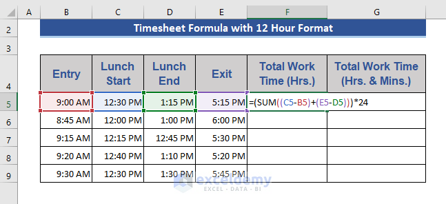
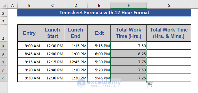
- Press Enter.
- Drag the Fill Handle icon down to fill the column.
- In Cell G5, enter the below formula:
=(C5-B5)+(E5-D5)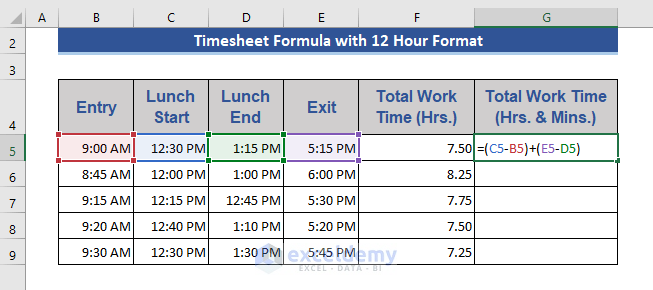
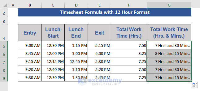
- Press Enter and drag the Fill Handle down to the last cell.
Get Total Work Time in a Week Considering Lunch Breaks
In a similar way to how we determined a timesheet for workdays with lunch breaks, we can determine the total working time of a week of workdays including lunch breaks.
Steps:
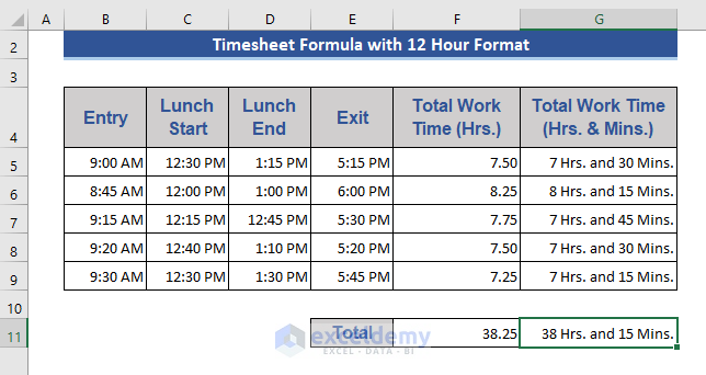
- Add a row named Total to the dataset like in the image below.
- Enter the below formula in Cell F11:
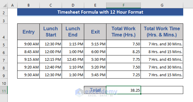
=SUM(F5:F9)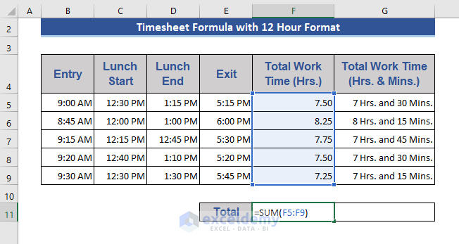
- Press Enter.
- Enter the following formula in Cell G11 and press Enter:
=SUM(G5:G9)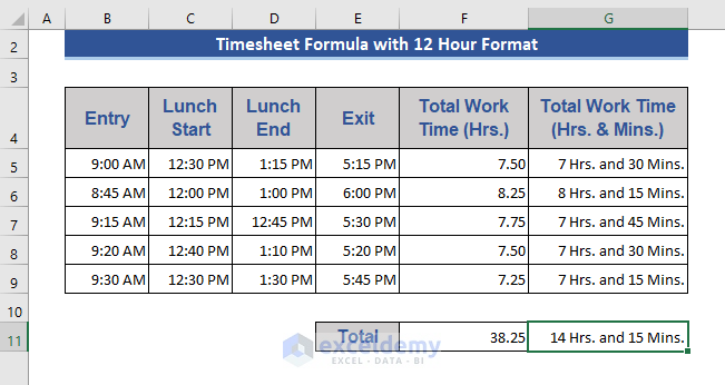
The result is not correct, because the value exceeds 24 hours.
- Click Ctrl+1 to open the Format Cells window.
- In the Type field enter: [h]” Hrs. and “m” Mins.”
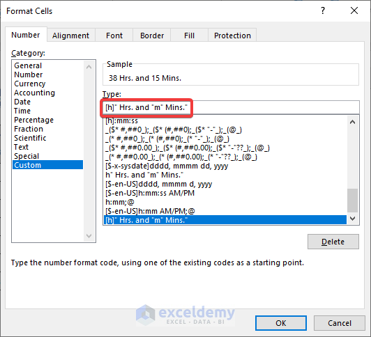
- Click OK.
The correct result in Hours and Minutes form is now displayed.
Download Practice Workbook
<< Go Back to Timesheet | Formula List | Learn Excel
Get FREE Advanced Excel Exercises with Solutions!
