Excel Conditional Formatting Based on Past or Due Date

Method 1 – Using Excel TODAY Function to Get Past or Due Date

Steps:

• Insert the following formula in Cell D5–

• Press ENTER for the output.

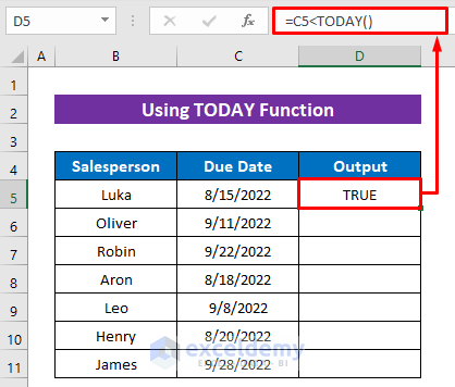
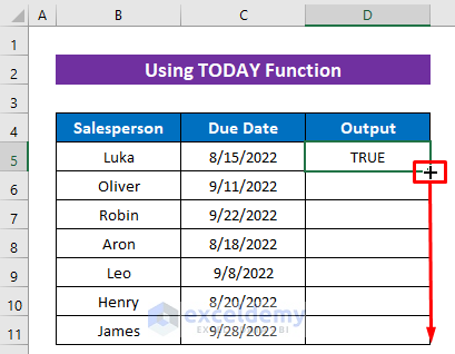
• Use the Fill Handle tool to copy the formula.

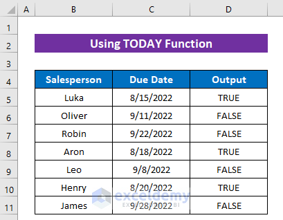
For the past or due dates, the result shows TRUE.

Method 2 – Use of Excel Conditional Formatting to Highlight Date Based on Past or Due Date

Steps:

• Select the date range.
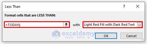
• Click as follows: Home > Conditional Formatting > Highlight Cells Rules > Less Than.

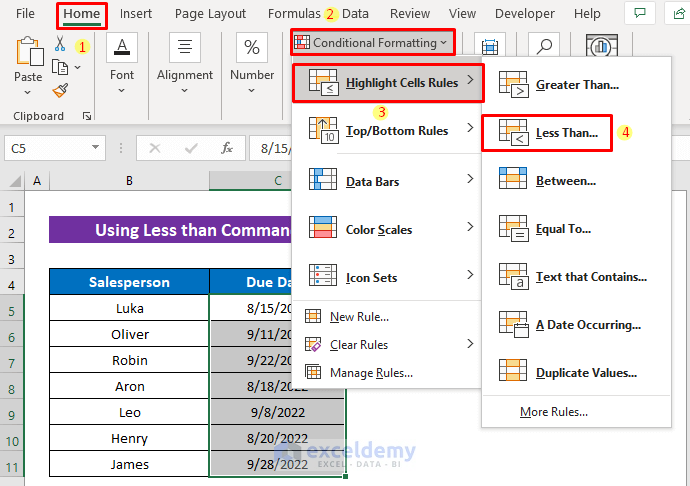
• Insert the following formula in the Format cells that are LESS THAN box:

• Choose the highlight color from the second box and press OK.

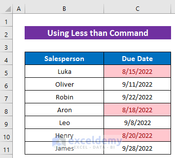
• The dates less than today will be highlighted with the selected color.

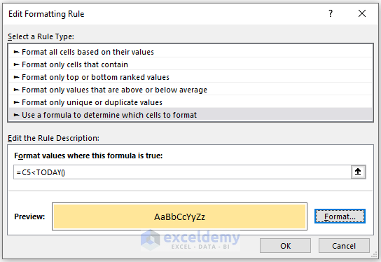
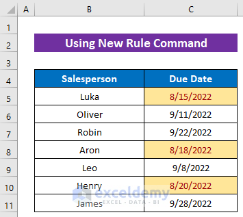
Method 3 – Using New Rule Command to Highlight Past Due Date in Excel

Steps:

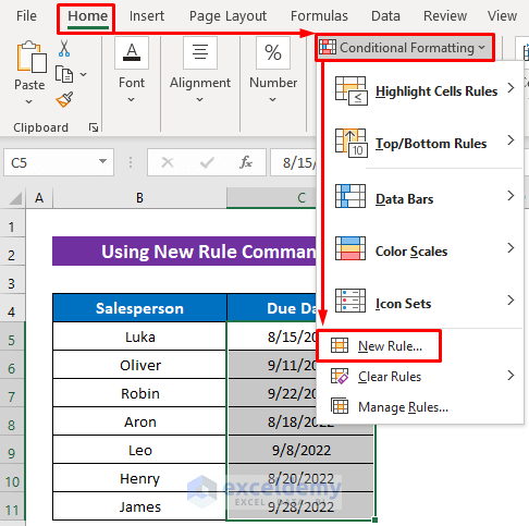
• Click as follows: Home > Conditional Formatting > New Rule.

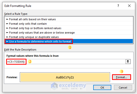
• Select Use a formula to determine which cells to format from the Select a Rule Type box.
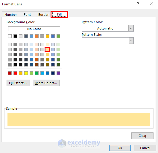
• Enter the following formula in the Format values where this formula is true box-

• Click the Format button. It will open the Format Cells dialog box.

• From the Fill section, choose a color.
• Click OK and it will take you back to the previous dialog box.

• Press OK.

The cells are now highlighted with the selected color.

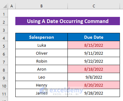
Method 4 – Applying ‘A Date Occurring’ Command to Highlight Date Past Due

Steps:

• Click as follows: Home > Conditional Formatting > Highlight Cells Rules > A Date Occurring.

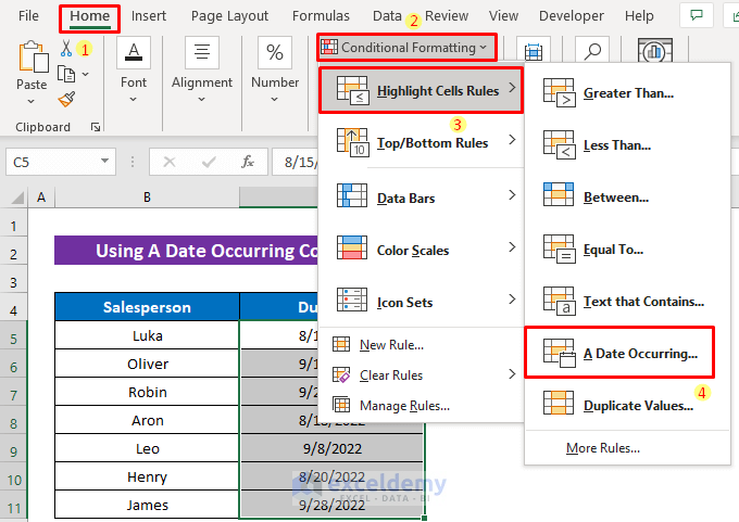
• From the first drop-down box, choose the right option for your dates.
• Select the highlight color from the second box and press OK.

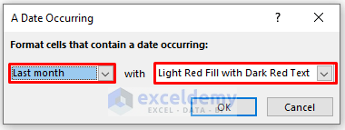
It highlights the past due dates of the last month.

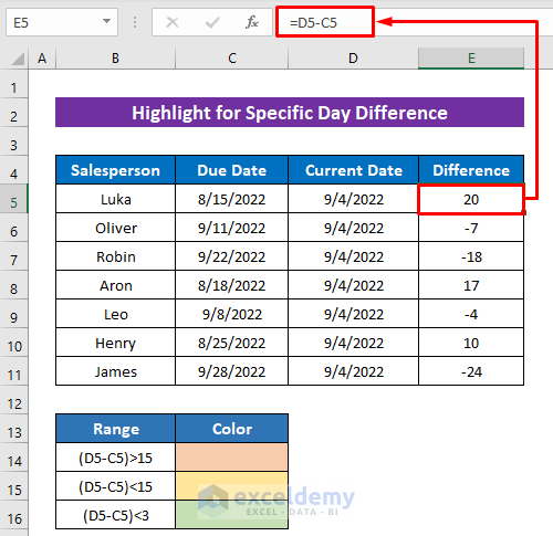
Method 5 – Highlighting Specific Day Differences for Date with Conditional Formatting in Excel

Find the day difference.

Steps:

• Insert the following formula in Cell E5 –

• Use the Fill Handle tool for the other cells.

• Select the dates from the Current Date column and f apply a rule.
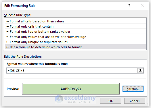
• Select Use a formula to determine which cells to format from the Select a Rule Type box.
• Enter the following formula in the Format values where this formula is true

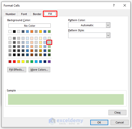
• Click the Format button. It will open the Format Cells dialog box.

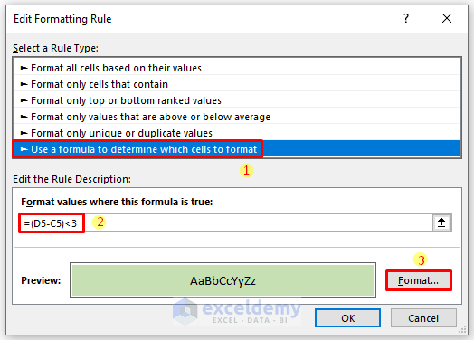
• Choose the fill color from the Fill
• Press OK.

• Return to the previous dialog box, press OK.

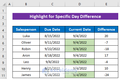
Here’s the output-

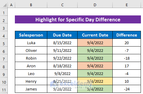
• Follow the same steps to apply the other two conditions.

Use the following formula for yellow color and biscuit color:

The final output will like this-

Download Practice Workbook

<< Go Back to Dates | Compare | Learn Excel