How to Apply Conditional Formatting to Dates 6 Months prior to Today – 3 Steps

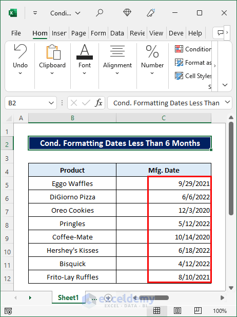
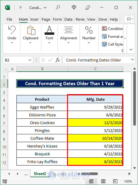
The dataset show cases products and manufacturing dates.

To highlight dates 6 months prior to today:

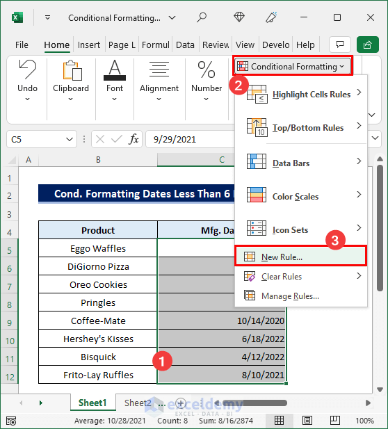
Step 1 – Select the Range and Add a New Rule

• Select the dates (C5:C12) and go to Home >> Conditional Formatting >> New Rule.

 Step 2 – Choose the Rule Type, Enter a Formula and Select a Fill Color

• Select Use a formula to determine which cells to format in Rule Type.
• Enter the following formula in the formula box.
• Click Format and choose a Fill color.
• Click OK.
• Click Apply, and OK again.

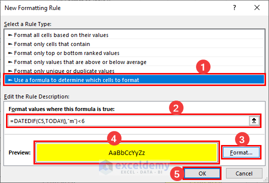
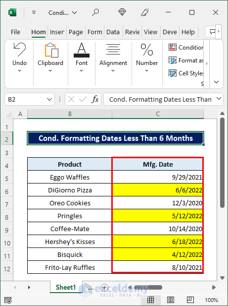
 Step 3 – Observe the Results

This is the output.

• You can also use the following formula:

Read More: How to Compare Dates in Two Columns in Excel

Conditional Formatting with Dates in Excel

Case 1: Applying Conditional Formatting to Dates Older Than 1 Year

• Use the following formula in the formatting rule.

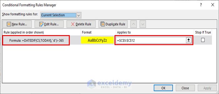
• You can also use the following formula:

This is the output.

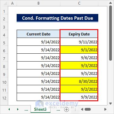
Case 2: Conditional Formatting Based on a Past Due Date

To apply conditional formatting and highlight the due dates within 10 days.

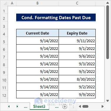
• Use the following formula in the conditional formatting rule for C5:C12.

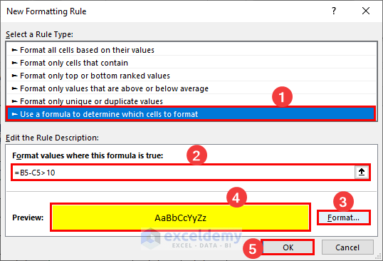
This is the output.

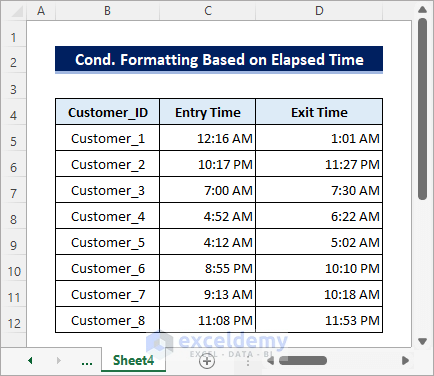
Case 3: Conditional Formatting Based on Elapsed Time

The dataset keeps record of the entry and exit times of customers in a shopping mall.

To find the customers who spent more than one hour in the mall:

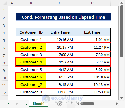
• Use the following formula in the formatting rule for B5:D12.

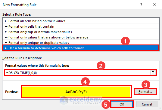
This is the output.

Things to Remember

• The TODAY function is a volatile function. It returns the current date and time every time you refresh the worksheet.

Download Practice Workbook

Download the practice workbook.

<< Go Back to Dates | Compare | Learn Excel