Dataset Overview
To illustrate these methods, let’s use a dataset containing the joining dates of 10 employees in a new startup company. Our dataset is located within the range of cells B5:C14.
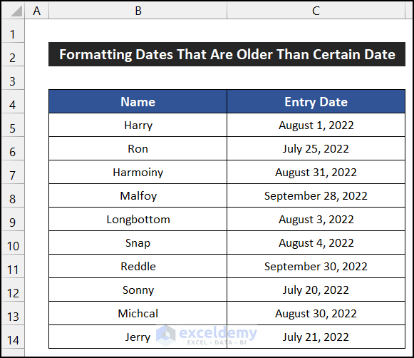
We need to figure out those employees who joined before August 29, 2022, or those dates that are older than August 29, 2022.
Method 1 – Using the DATE Function
In this method, we’ll utilize the DATE function to apply conditional formatting for dates older than a specified date. Follow these steps:
Steps:
- Select the range of cells C5:C14.
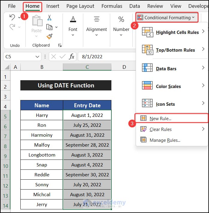
- Go to the Home tab, click the drop-down arrow of Conditional Formatting and select New Rules in the Styles group.
- A dialog box named New Formatting Rule will appear.
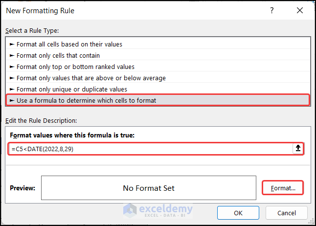
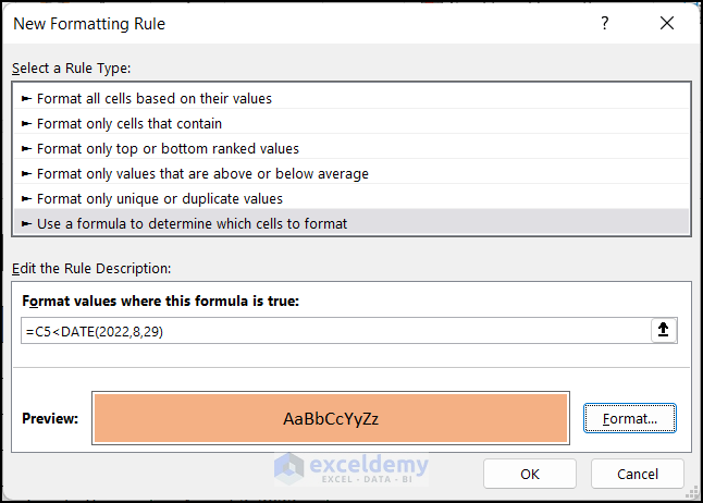
- Select the Use a formula to determine which cells to format option.
- In the empty box below the text, Formula values where this formula is true, enter the following formula:
=C5<DATE(2022,8,29)
- Click the Format option.
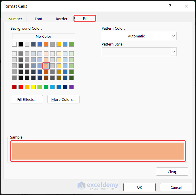
- Another dialog box titled Format Cells will appear.
- Set the cell formatting according to your preference. For example, choose the Orange, Accent 2, Lighter 40% color from the Fill tab.
- Click OK to close the Format Cells dialog box.
- Click OK again to close the New Formatting Rule dialog box.
- You’ll see that the dates older than August 29, 2022, are highlighted.
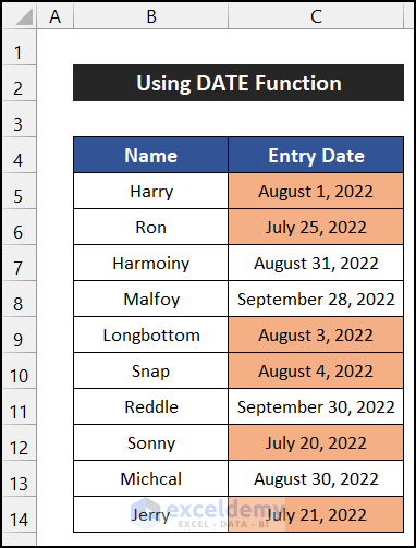
This confirms that the formula is working correctly, and conditional formatting for dates older than a specific date is applied successfully.
Method 2 – Using the TODAY Function
In this approach, we’ll use the TODAY function to apply conditional formatting for dates older than the current date. Follow these steps:
Steps:
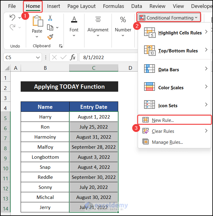
- Select the range of cells C5:C14.
- In the Home tab, click the drop-down arrow of Conditional Formatting and select New Rules in the Styles group.
- The New Formatting Rule dialog box will appear.
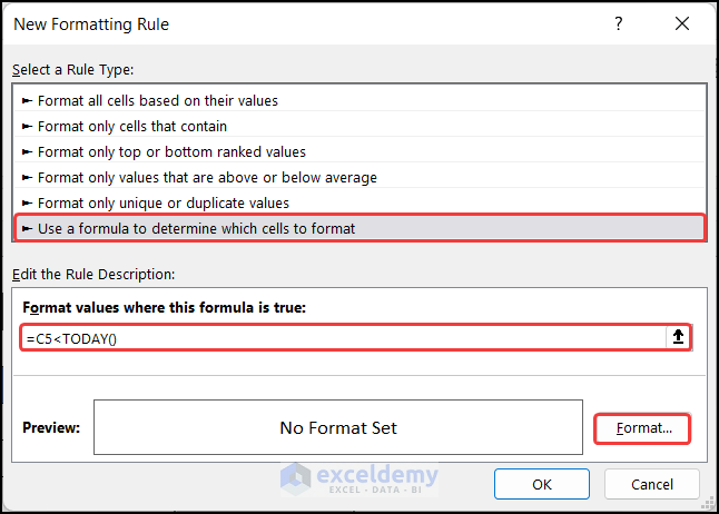
- Select the Use a formula to determine which cells to format option.
- In the empty box below the text, Formula values where this formula is true, enter the following formula:
=C5<TODAY()
- Click the Format option.
- Another dialog box named Format Cells will appear.
- Set the cell formatting according to your preference. For instance, choose the Orange, Accent 2, Lighter 40% color from the Fill tab.
- Click OK to close the Format Cells dialog box.
- Click OK again to close the New Formatting Rule dialog box.

- You’ll observe that dates older than the current date are highlighted.
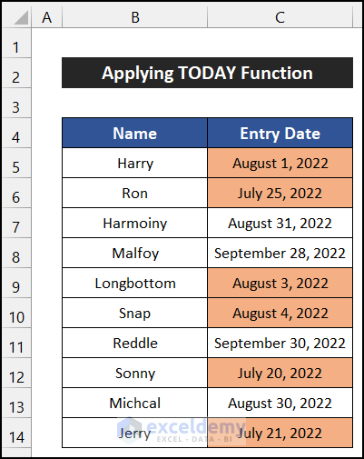
This demonstrates that the formula is effective, and conditional formatting for dates older than the current date is successfully applied.
Method 3 – Using the DATEVALUE Function
In this process, we’ll utilize the DATEVALUE function to apply conditional formatting for dates older than a specified date. Follow these steps:
Steps:
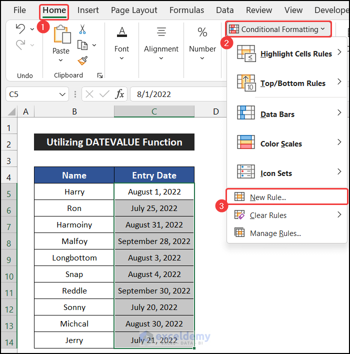
- Select the range of cells C5:C14.
- Go to the Home tab, then click the drop-down arrow of Conditional Formatting and select New Rules in the Styles group.
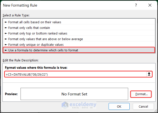
- A small dialog box titled New Formatting Rule will appear.
- Select the Use a formula to determine which cells to format option.
- In the empty box below the text, Formula values where this formula is true, enter the following formula:
=C5<DATEVALUE("08/29/22")
- Click the Format option.
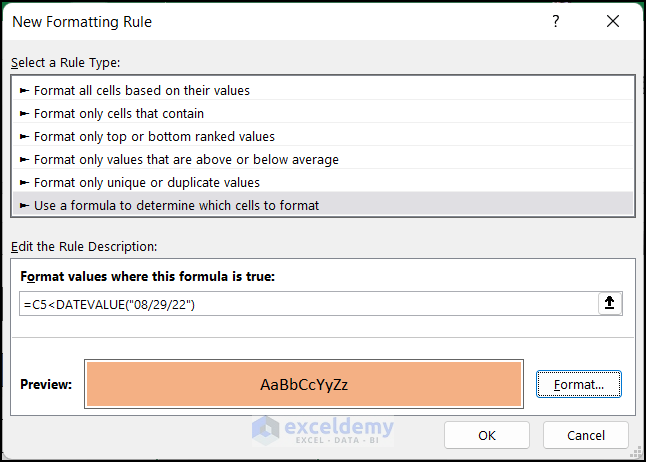
- Another dialog box named Format Cells will appear.
- Set the cell formatting according to your preference. For example, choose the Orange, Accent 2, Lighter 40% color from the Fill tab.
- Click OK to close the Format Cells dialog box.
- Click OK to close the New Formatting Rule dialog box.
- You’ll see that the dates older than August 29, 2022, are highlighted.

This confirms that the formula works accurately, and conditional formatting for dates older than a specific date is applied successfully.
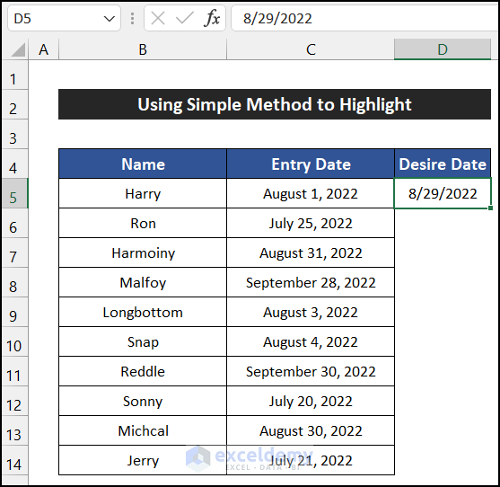
Method 4 – Using a Simple Method for Highlight
In this case, we’ll employ a straightforward method to apply conditional formatting for dates older than a certain date. Follow these steps:
Steps:
- In cell D5, enter your desired date (e.g., August 29, 2022).
- Change the number format of that cell from Date to General to obtain the date value from the Number group.
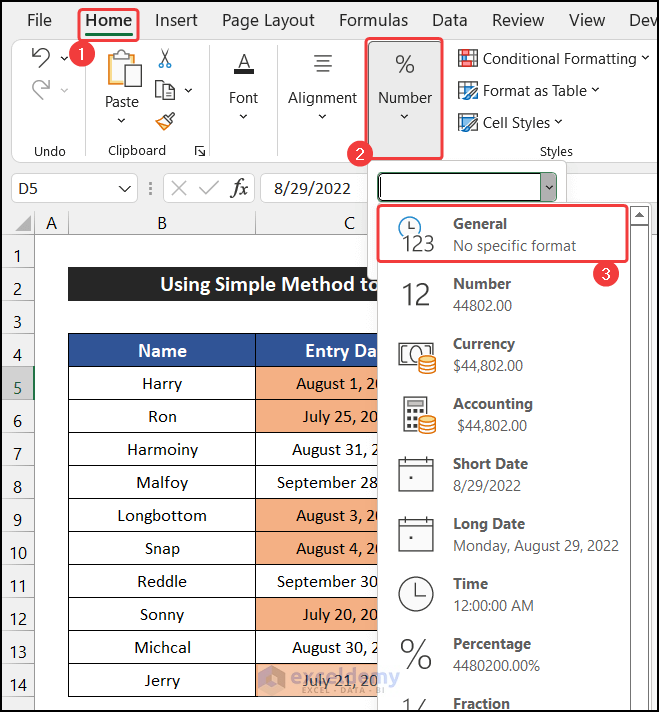
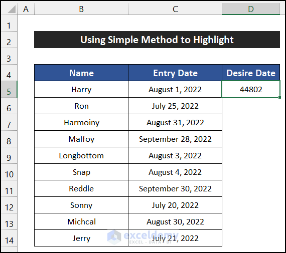
- You’ll receive the date value in General format, which is 44802.
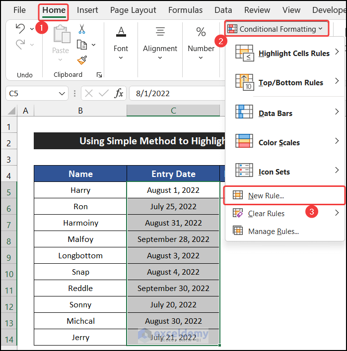
- Select the range of cells C5:C14.
- In the Home tab, click on the drop-down arrow of the Conditional Formatting and select New Rules option located in the Styles group.
- A small dialog box named New Formatting Rule will appear.
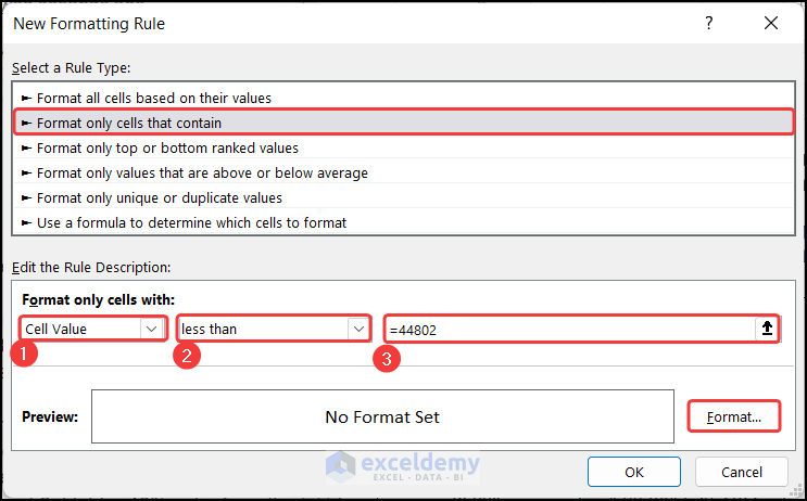
- Select the option called Format only cells that contain.
- Set the features according to your preference.
- In the first field, set the Cell Value.
- In the second field, set the option titled less than.
- In the last field, enter the date value.
=44802
- Click the Format option.
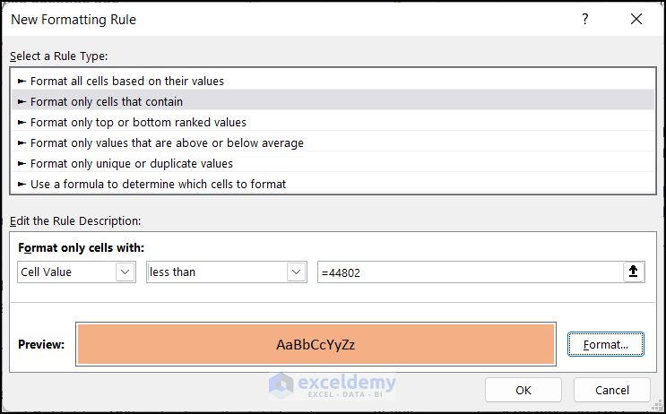
- Another dialog box named Format Cells will appear.
- Set the cell formatting according to your preferences. For instance, choose the Orange, Accent 2, Lighter 40% color from the Fill tab.
- Click OK to close the Format Cells dialog box.
- Click the OK again to close the New Formatting Rule dialog box.
- You’ll observe that dates older than August 29, 2022, are highlighted.
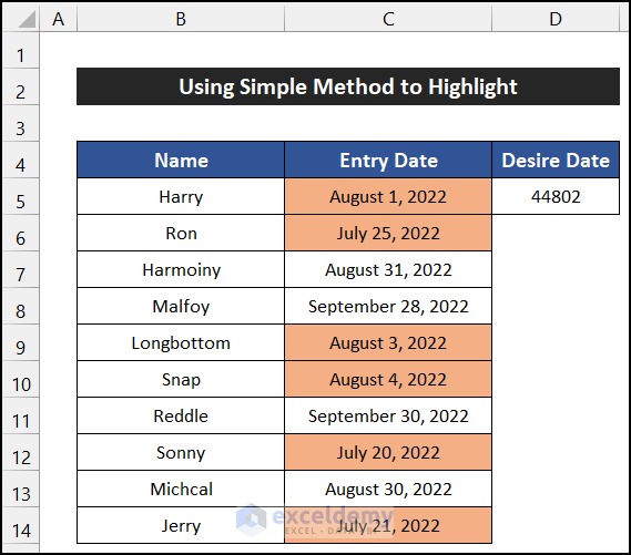
We can conclude that our method works effectively, and conditional formatting for dates older than a certain date is successfully applied.
Method 5 – Customizing New Rules with Defined Cell Reference
In this approach, we’ll customize the New Rules option to apply conditional formatting for dates older than a certain date using a defined cell reference. Follow these steps:
Steps:
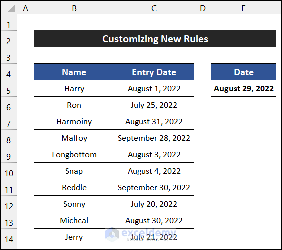
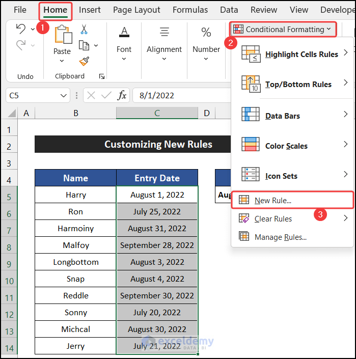
- In cell E5, enter your desired date (e.g., August 29, 2022).
- Select the range of cells C5:C14.
- In the Home tab, click on the drop-down arrow of the Conditional Formatting and select New Rules in the Styles group.
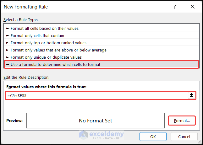
- A small dialog box named New Formatting Rule will appear.
- Select the Use a formula to determine which cells to format option.
- In the empty box below the text, Formula values where this formula is true, enter the following formula:
=C5<$E$5
- Click the Format option.
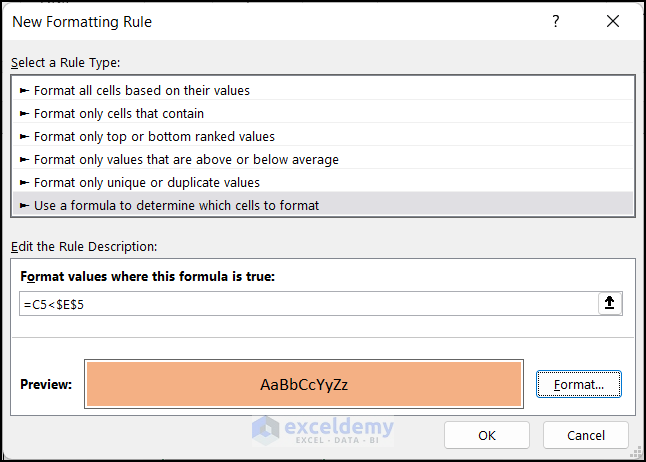
- Another dialog box named Format Cells will appear.
- Set the cell formatting according to your preferences. For example, choose the Orange, Accent 2, Lighter 40% color from the Fill tab.
- Click OK to close the Format Cells dialog box.
- Click OK again to close the New Formatting Rule dialog box.
- You’ll notice that dates older than August 29, 2022, are highlighted.
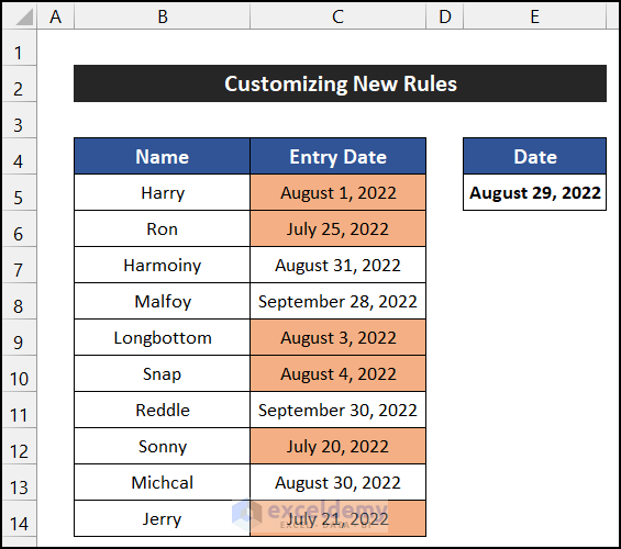
Our approach works perfectly, and we can apply conditional formatting for dates older than a certain date using this method.
Download Practice Workbook
You can download the practice workbook from here:
<< Go Back to Dates | Compare | Learn Excel
Get FREE Advanced Excel Exercises with Solutions!
