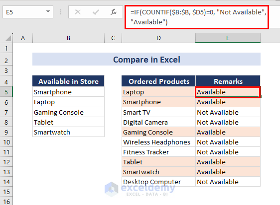
In the following overview image, we have compared two different lists containing the available products in a store and ordered products. If the ordered products are in the list of available products, they are remarked as “Available” and if they are not in the list, they are remarked as “Not Available”.
⏷Compare Two Columns Row-by-Row
⏵Compare Numeric Values
⏵Compare Text Strings (Case Sensitive/Insensitive)
⏵Comparing Date Values in Excel
⏷Compare Multiple Columns for Row Matches
⏷Compare Two Lists for Similarities and Differences
⏷Compare Two Lists and Pulling Matched Data
⏷Compare and Highlight Row Similarities and Differences
⏷Compare Any 2 Cells and Write Remarks in Excel
⏷Comparing 2 Columns in Different Sheets
⏷Comparing 2 Different Excel Workbooks
⏷Statistical Comparison in Excel
⏷Using VBA to compare 2 Columns Based on User Input
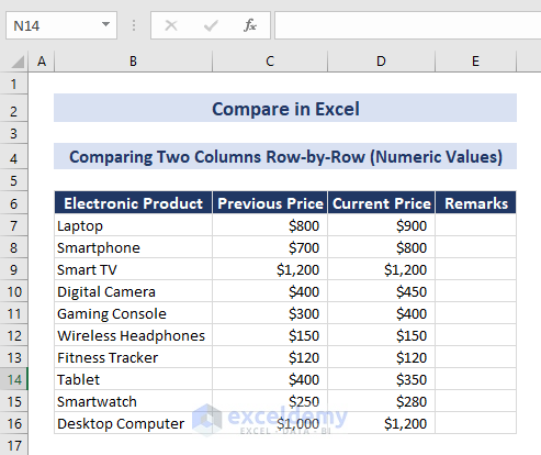
Method 1 – Compare Two Columns Row-by-Row in Excel
Case 1.1 – Compare Numeric Values
In the following dataset, we have a list of 10 electronic products along with their current and previous prices listed accordingly. Now we will compare these prices and evaluate whether the prices have changed or not.
Steps:
- Inside cell E7 copy the following formula:
=IF(C7=D7,"No Change","Change")- Press Enter. This will return “Change” if the prices are not the same or return “No Change” if the prices remain constant.
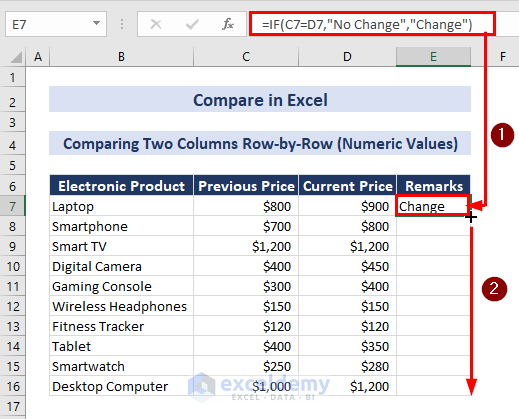
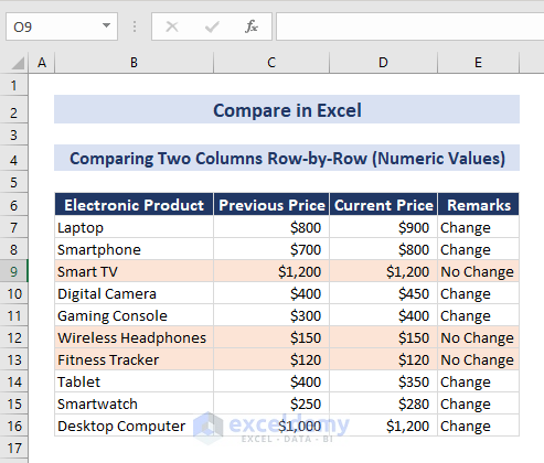
- Use the Fill Handle to copy the formula in the other cells below.
The rows with “No Change” remarks have been highlighted in the sample for better visualization.
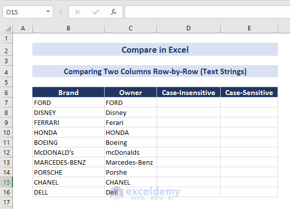
Case 1.2 – Compare Text Strings (Case Sensitive/Insensitive)
In the dataset below, we have taken a list of famous brands and the names of their owners. All the brand names are given after their owners’ names. We will compare these text strings and evaluate if the strings are matched or not.
Steps:
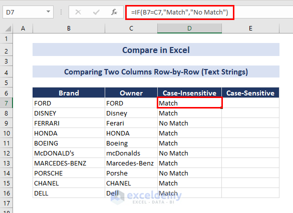
- Copy the following formula inside cell D7 for a case-insensitive match:
=IF(B7=C7,"Match","No Match")- Press Enter and use AutoFill to copy the formula down.
Only the misspellings will result in “No Match”. Otherwise, all the names are matched regardless of their case sensitivity.
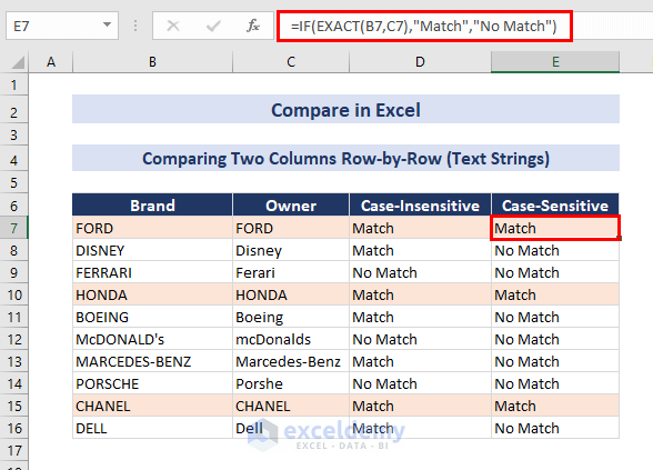
- To compare case-sensitive text strings, use the formula:
=IF(EXACT(B7,C7),"Match","No Match")Only the exact matches with the right spellings and case sensitivities are matched.
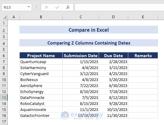
Case 1.3 – Comparing Date Values in Excel
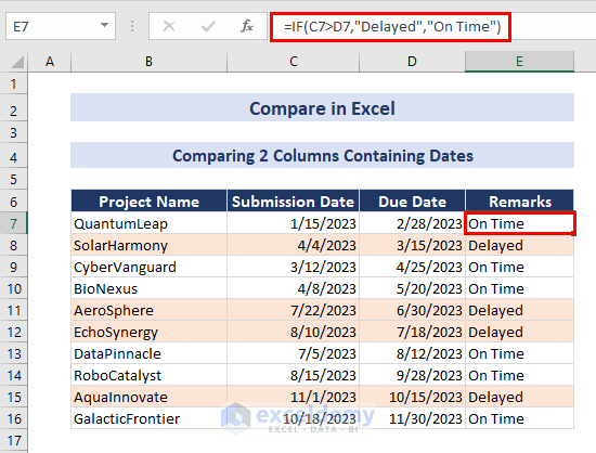
In the following dataset, we have a list of 10 projects along with their due dates and submission dates. Let’s compare these dates and evaluate if the projects were submitted before the deadlines or not.
Steps:
- Put the following formula inside cell E7:
=IF(C7>D7,"Delayed","On Time")- Press Enter and use the Fill Handle to copy the formula into the rest of the cells.
The projects that were submitted before the deadline are remarked with “On Time”. And the projects that were submitted past the due date are remarked with “Delayed”.
Method 2 – Compare Multiple Columns for Row Matches
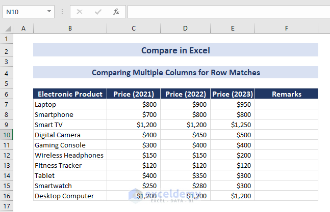
In the following dataset, we have a list of 10 electronic products along with their prices in the years 2021, 2022, and 2023. Let’s compare these 3 columns in Excel and evaluate whether these prices are fully stable, almost stable, or unstable.
Steps:
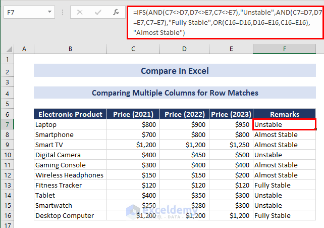
- Input the following formula inside cell F7:
=IFS(AND(C7<>D7,D7<>E7,C7<>E7),"Unstable",AND(C7=D7,D7=E7,C7=E7),"Fully Stable",OR(C16=D16,D16=E16,C16=E16),"Almost Stable")- Press Enter and use Autofill to copy the formula down.
The prices that are different in all 3 years are remarked as “Unstable”.
The prices that are constant throughout any two years and different in only one year are remarked as “Almost Stable”.
Finally, the prices that have remained constant for all three years are remarked as “Fully Stable”.
Method 3 – Compare Two Lists for Similarities and Differences in Excel
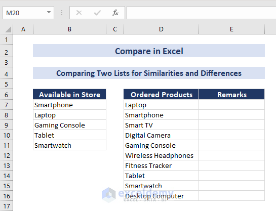
In the dataset below, we have two separate lists. One contains the ordered products, and the other contains the products that are currently available in the store. Let’s compare these lists and determine which ordered products are currently available in the store.
Steps:
- Inside cell E7, copy the following formula:
=IF(COUNTIF($B:$B, $D7)=0, "Not Available", "Available")- Press Enter and use the Fill Handle to copy the formula in the other cells below.
The available products are highlighted for better visualization.
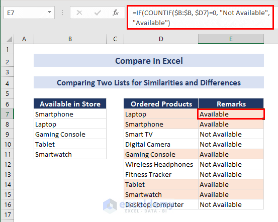
Now, if any new item is listed as available in the store (by putting a new row and entering the value) and matches the list of ordered products, it will be automatically marked as “Available” as well as highlighted.
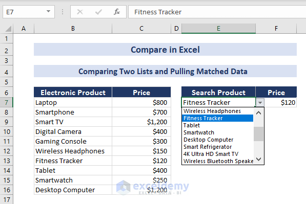
Method 4 – Compare Two Lists and Pulling Matched Data
We have a list of 10 electronic products along with their prices in the following dataset. In cell E7, we will make a drop-down list in Excel with some product names that are not all available in the Electronic Product list. Now, we will select any of the products from the search product list to compare their value with the electronic product lists. For any matched value in the following lists, it will pull the price data of the electronic product, and for any unmatched value, it will return “Not Available”.
Steps:
- Inside cell F7, copy the following formula:
=IFERROR(VLOOKUP(E7,B7:C16,2,FALSE),"Not Available")- Press Enter.
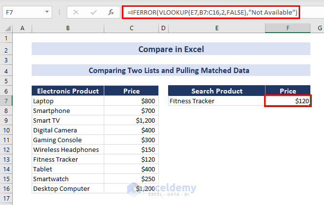
The following GIF shows the corresponding prices getting changed as we select different products. If we select a product that is not included in the given list, it will show “Not Available”.

Note: We can alternatively use any of the following two formulas:
=XLOOKUP(E7,B7:B16,C7:C16,,0)Or,
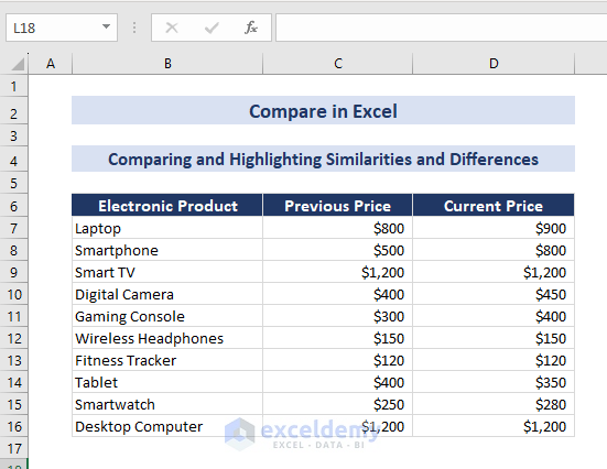
=INDEX(B7:C16,MATCH(E7,B7:B16,0),2)Method 5 – Compare and Highlight Row Similarities and Differences
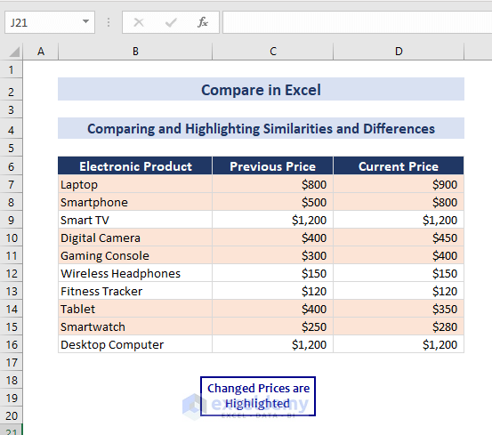
In the dataset below, we have a column containing the previous price and another column containing the current prices of 10 electronic items. Let’s compare these columns and highlight the rows containing the products with changed prices.
Steps:
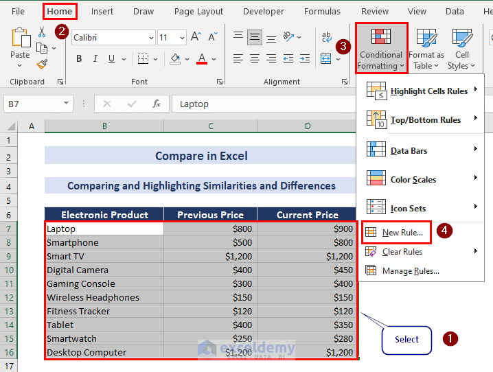
- Select the range B7:D16.
- Go to Home, select Conditional Formatting in the Styles group, and choose New Rule…
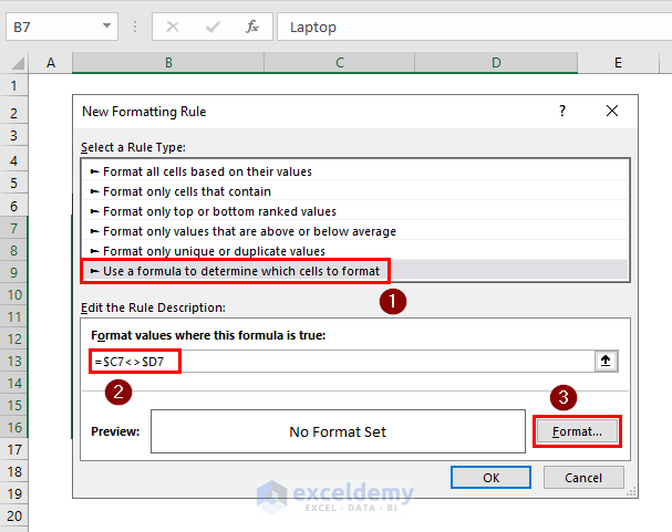
- A dialogue box named New Formatting Rule pops out.
- Under Select a Rule Type:, select Use a formula to determine which cells to format.
- Under Format values where this formula is true:, copy the following formula:
=$C7<>$D7- Click on Format…
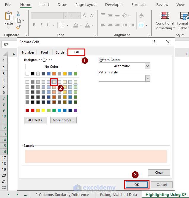
- A new dialogue box named Format Cells pops out.
- Click on the Fill tab and select any suitable fill color.
- Click on OK.
- Click on OK inside the New Formatting Rule dialogue box.
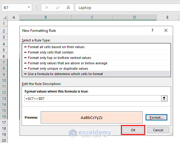
- This highlights the rows containing the products with the changed prices.
Method 6 – Compare Any 2 Cells and Write Remarks in Excel
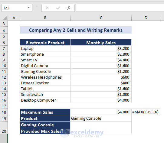
In the following dataset, we have a list of 10 electronic products along with their monthly sales. The cell C18 holds the value of the maximum sales.
The formula for calculating the maximum sales is:
=MAX(C7:C16)Now we will compare the maximum sales in C18 with the sales of the selected product from the drop-down list in cell C19 and get the correct remark.
Steps:
- Copy the following formula inside cell C20:
=IF(VLOOKUP(C19,B7:C16,2,FALSE)=C18,"Yes", "No")- Press Enter.
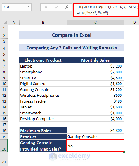
- The following GIF shows that the remark changes by comparing two cells as we select different products.
Method 7 – Compare 2 Columns in Different Excel Worksheets
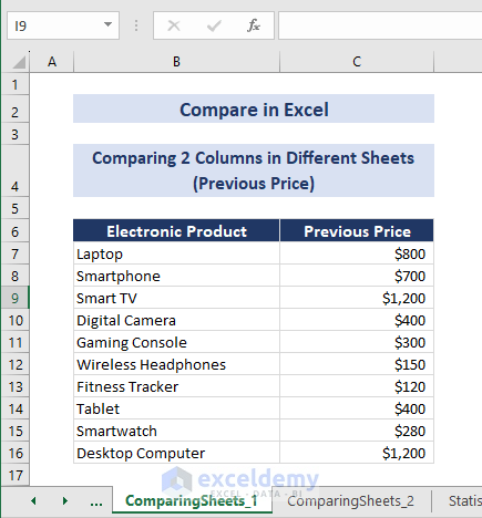
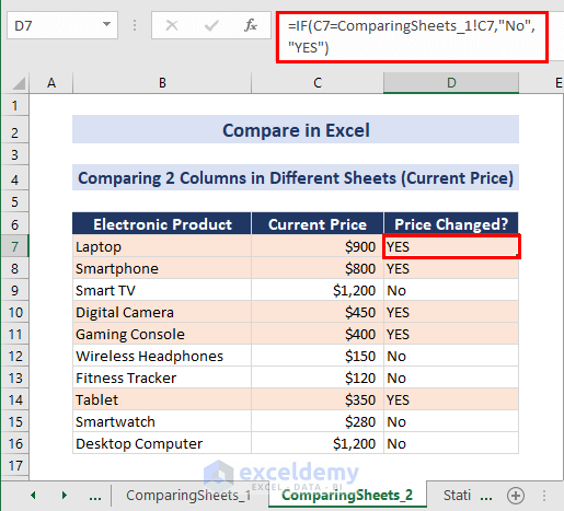
In the dataset below, we have the previous prices of 10 electronic products in one worksheet and the current prices of the same products in another worksheet. Let’s determine whether the prices have changed or not.
Steps:
- Go to the ComparingSheets_2 sheet.
- Select cell D7.
- Input the following formula:
=IF(C7=ComparingSheets_1!C7,"No","YES")- Press Enter and use the Fill Handle to copy the formula into the rest of the cells.
The current prices that are different from the previous prices are remarked with “Yes” and the current prices that are similar to the previous prices are remarked with “No”.
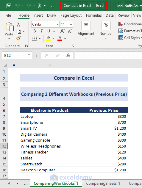
Method 8 – Compare 2 Different Workbooks in Excel
In the dataset below, we have the previous prices of 10 electronic products in one workbook and the current prices of the same products in another workbook.
Steps:
- Go to the Compare in Excel Sub1 workbook and the Comparing Workbooks_2 worksheet.
- Select cell D7 and insert the following formula:
=IF(C7='C:\Users\Gadget 360\Desktop\[Compare in Excel.xlsm]ComparingWorkbooks_1'!C7,"No","YES")- Press Enter and use the Fill Handle to copy the formula into the rest of the cells.
The current prices that are different from the previous prices are remarked with “Yes” and the current prices that are similar to the previous prices are remarked with “No”.
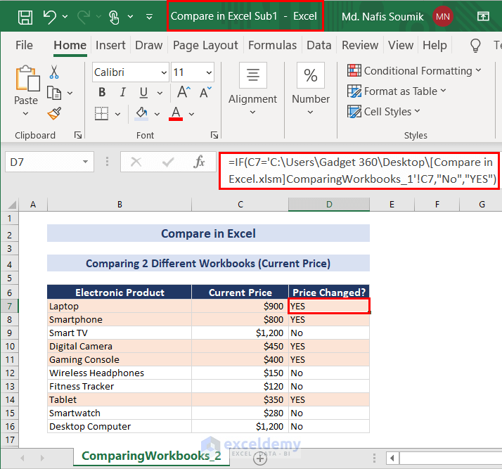
Note: In the formula inside the IF function, we have used the folder path appropriate for us. However, the users should use their own folder path where the files are actually located. For best results, we recommend putting the files in the same folder, which allows you to omit the folder path and just input the file name and extension.
Method 9 – Statistical Comparison in Excel
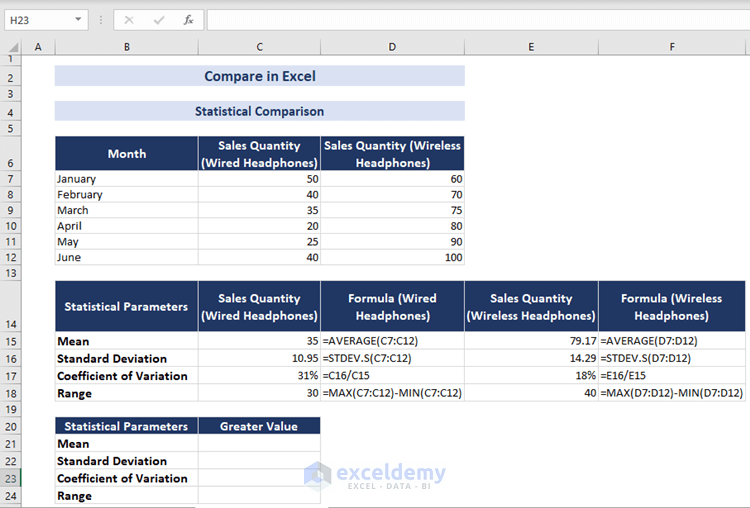
In the following dataset, we have six monthly sales quantities of wireless and wired headphones in two different columns. We will calculate the Mean, Standard Deviation, Coefficient of Variation, and Range of these two different lists.
To calculate the Mean of Wired Headphones use the formula below:
=AVERAGE(C7:C12)The formula to calculate the Standard Deviation of Wired Headphones is:
=STDEV.S(C7:C12)To calculate the Coefficient of Variation of Wired Headphones use the formula below:
=C16/C15To calculate the Range of Wired Headphones use the formula below:
=MAX(C7:C12)-MIN(C7:C12)We have also calculated the Mean, Standard Deviation, Coefficient of Variation, and Range for the Wireless Headphones.
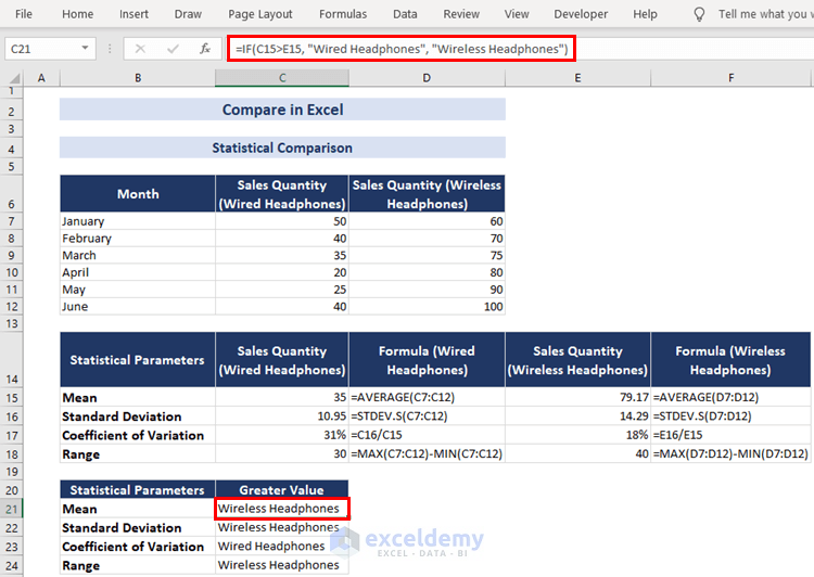
Steps:
- Put the following formula inside cell C19:
=IF(C15>D15, "Wired Headphones", "Wireless Headphones")- Press Enter and use the Fill Handle to copy the formula into the rest of the cells.
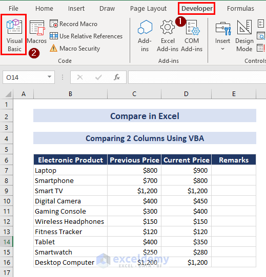
Method 10 – Comparing 2 Columns Based on User Input Using Excel VBA
Let’s make a form where the users will enter the column names to compare and then input the column name where they want to get the output.
Steps:
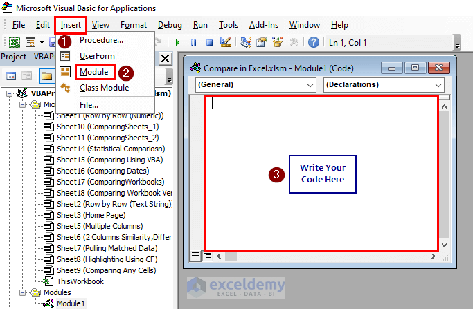
- Click on Developer and select Visual Basic.
- A new window named Microsoft Visual Basic for Applications will open.
- Inside the Visual Basic window, click on Insert and select Module.
- A blank module will open for you to write the VBA code.
- Inside the module, copy the following code:
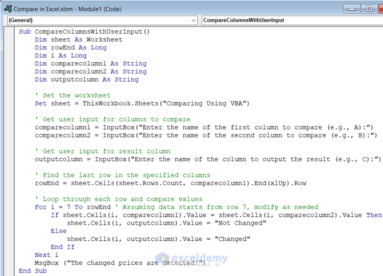
Code Syntax:
Sub CompareColumnsWithUserInput()
Dim sheet As Worksheet
Dim rowEnd As Long
Dim i As Long
Dim comparecolumn1 As String
Dim comparecolumn2 As String
Dim outputcolumn As String

' Set the worksheet
Set sheet = ThisWorkbook.Sheets("Comparing Using VBA")

' Get user input for columns to compare
comparecolumn1 = InputBox("Enter the name of the first column to compare (e.g., A):")
comparecolumn2 = InputBox("Enter the name of the second column to compare (e.g., B):")

' Get user input for result column
outputcolumn = InputBox("Enter the name of the column to output the result (e.g., C):")

' Find the last row in the specified columns
rowEnd = sheet.Cells(sheet.Rows.Count, comparecolumn1).End(xlUp).Row

' Loop through each row and compare values
For i = 7 To rowEnd ' Assuming data starts from row 7, modify as needed
If sheet.Cells(i, comparecolumn1).Value = sheet.Cells(i, comparecolumn2).Value Then
sheet.Cells(i, outputcolumn).Value = "Not Changed"
Else
sheet.Cells(i, outputcolumn).Value = "Changed"
End If
Next i
MsgBox ("The changed prices are detected!")
End Sub
- Save the file and close the Visual Basic window.
- Click on Developer and select Macros.
- Inside the dialogue box named Macro, select the code you have just written and click on Run.
- Three dialogue boxes will appear one by one. In the first two dialog boxes, we will input the two column names to compare. In the last dialog box, we’ll input the column name where we want to get the output.
This will remark the changed prices as “Changed” and the unchanged prices as “Not Changed”. Changed prices are highlighted for better visualization.
Download Practice Book
Compare in Excel: Knowledge Hub
<< Go Back to Learn Excel
Get FREE Advanced Excel Exercises with Solutions!
