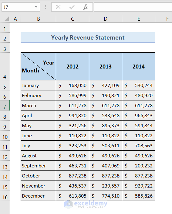
We have used a sample yearly revenue statement to demonstrate 4 methods to compare 3 columns for matches in Excel. We will find the matchings among columns C, D, and E while discussing the methods below.
Method 1 – Compare 3 Columns in Excel for Matches Using the IF Function along with AND Function
Steps:
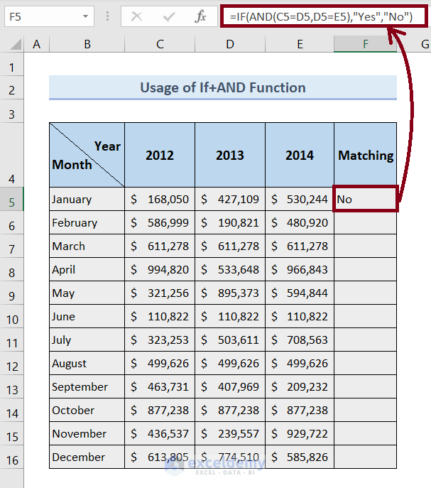
- Select Cell F5 to store the matching result.
- Copy the following formula:
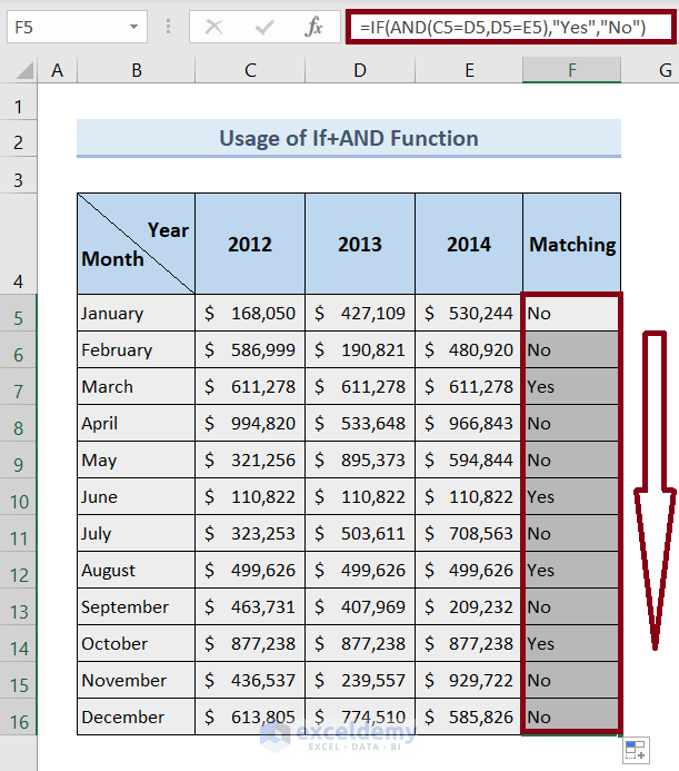
=IF(AND(C5=D5,D5=E5),"Yes","No")- Press Enter.
- Drag the Fill Handle icon to the end of column F.
Method 2 – Highlight the Matching Data by Juxtaposing 3 Columns in Excel by Setting Up New Rule
Steps:
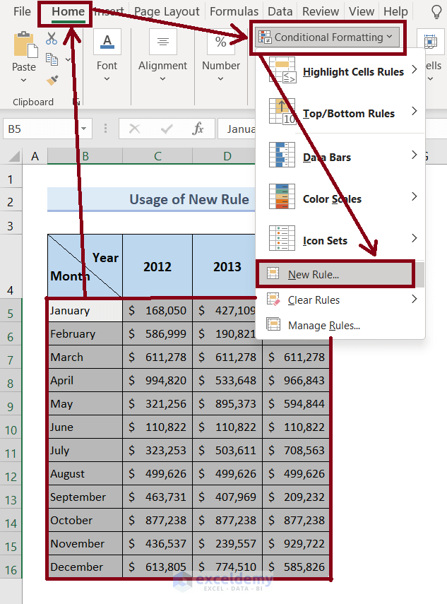
- Select the whole dataset.
- Go to the Home ribbon.
- Click on the Conditional Formatting.
- From the drop-down menu, select New Rule.
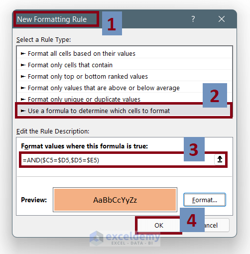
- The New Formatting Rule window will pop up.
- Select Use a formula to determine which cells to format.
- In the formula box, copy:
=AND($C5=$D5,$D5=$E5)- Press the OK button.
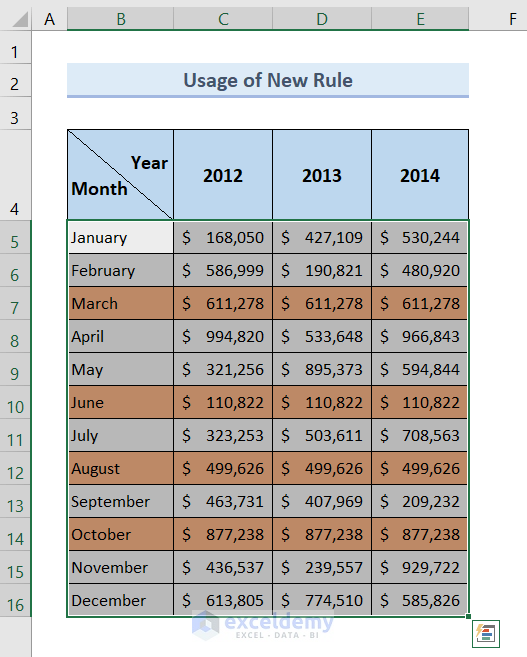
When you are done, you will get all the matched data highlighted.
Method 3 – Compare 3 Columns for Matches in Excel Using IF with COUNTIF Function
Steps:
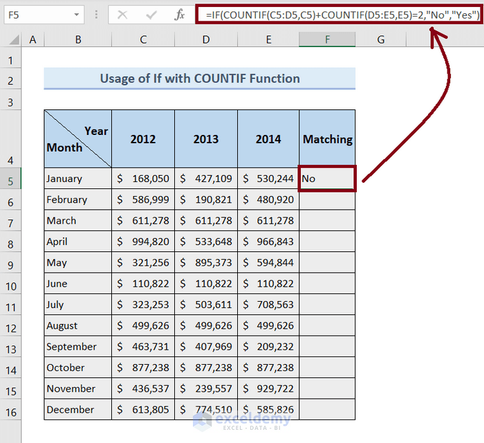
- Select Cell F5.
- Copy the following formula into the cell:
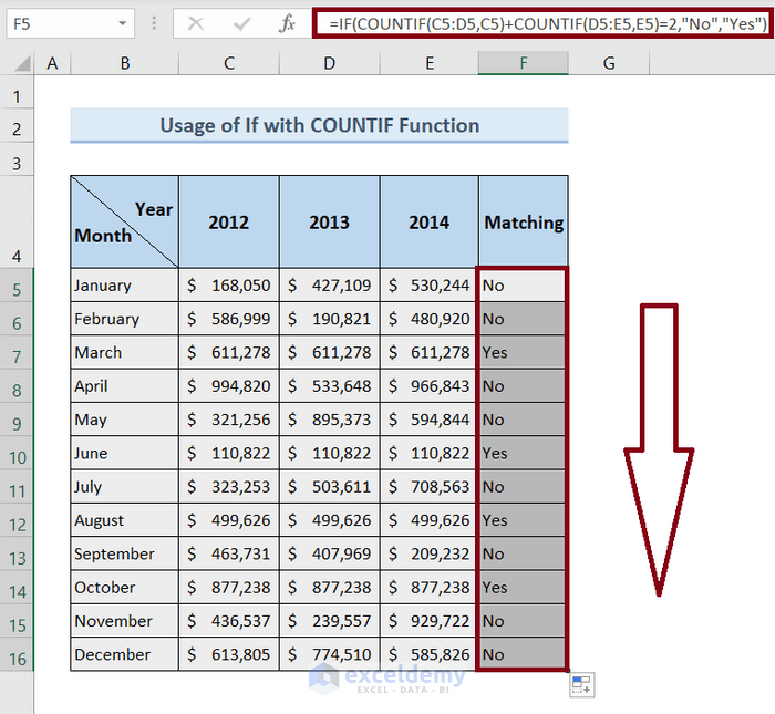
=IF(COUNTIF(C5:D5,C5)+COUNTIF(D5:E5,E5)=2,"No","Yes")- Press Enter.
- Drag the Fill Handle icon to the end of column F.
Method 4 – Highlight the Matched Records by Scanning 3 Columns in Excel
You can use the Duplicate Values option under the Conditional Formatting option to highlight the matching records in Excel.
Steps:
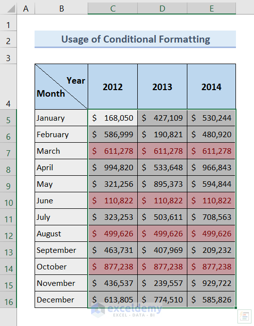
- Select columns C, D, and E.
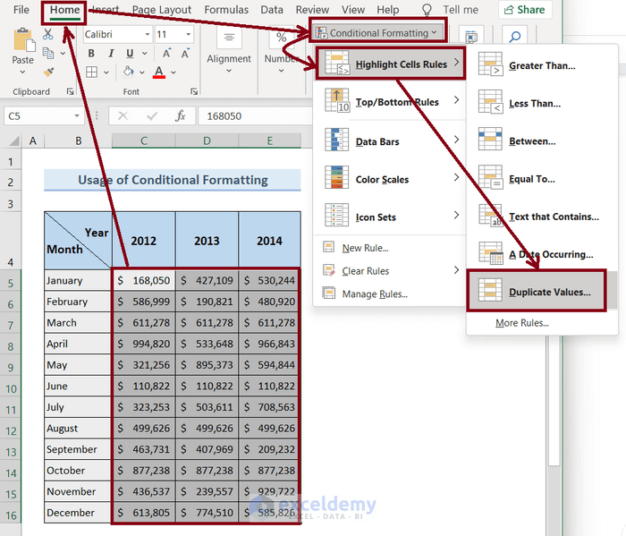
- Go to the Home ribbon.
- Click on the Conditional Formatting.
- Navigate to the Highlight Cells Rules option.
- Select the Duplicate Values… option from the drop-down list.
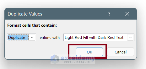
- A new window named Duplicate Values will open. Hit the OK button in it.
- You will get all the matched records being highlighted like this:
Things to Remember
Always be careful while inserting range within the formulas.
Select the dataset first before moving into Conditional Formatting.
Don’t forget to pick up the color to format cells while using Conditional Formatting.
Download the Practice Workbook
You are recommended to download the Excel file and practice along with it.
<< Go Back to Columns | Compare | Learn Excel
Get FREE Advanced Excel Exercises with Solutions!

Hi Mrinmoy, thank you for your excel tips. I need help to compare three columns between multiple sheets and find the same values and give me yes or no result. Please can you help. Thanks.
Hello Mr. Masud,
You can easily solve your problem by combining the IF and AND functions.
Suppose, you have 3 values to compare in three cells C7, D7, and E7. For this instance, let’s say C7 is in sheet1, D7 is in sheet2, and E7 is in sheet3.
Now you are in sheet3 and you want to get a feedback (Yes or No) in cell F7.
All you need to do is, type the following formula in cell F7 of sheet3.
=IF(AND(Sheet1!C7=Sheet2!D7,Sheet2!D7=Sheet3!E7),”Yes”,”No”)
After that, press ENTER and you will get your required result.
Regards!
Hello Mrinmoy, thank you for your excel tips. I need help to solve this problem. There are two workbooks containing numbers in column A and some other value in column Z against these numbers in each row, in both the workbooks. I need to compare the numbers in column A in both workbooks and if they match, copy values from column Z in first workbook against column A numbers in second workbook, wherever numbers in column A of both workbooks match. I would highly appreciate, if you could help me in this regard.
Hello Murali,
Unfortunately, I find your query a little confusing. It would’ve been much better if you had explained it with sample data and desired outputs.
As far as I understand, you need to compare column A in Book1 to column A in Book2. So, you want to create a formula in Book2 so that, if there is a match, it will return the corresponding value from column Z in Book1.
You can apply the following formula to do that. Then copy the formula down.
=IF(Sheet1!A1=[Book1.xlsx]Sheet1!A1,[Book1.xlsx]Sheet1!Z1,"")Is this what you wanted? I’ve also emailed you the Excel documents. Please check.
Thanks for being with us.
Regards,
Md. Shamim Reza (ExcelDemy Team)