Method 1 – Using Conditional Formatting
Steps:
- Select the cells of 4 Columns from the dataset.

- Go to the Home tab.
- Select the Conditional Formatting from the commands.
- Select Duplicate Values from Highlight Cells Rules.
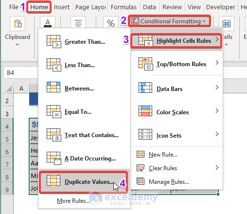
- You will get a Pop-Up.
- Select Duplicate Values and your desired color.
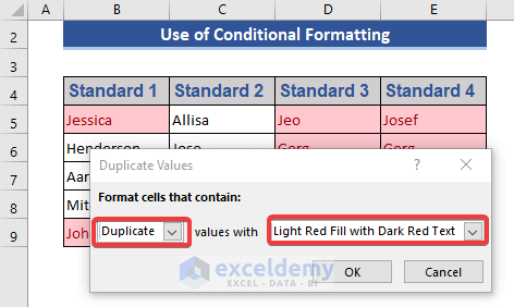
- Press OK to get the result.
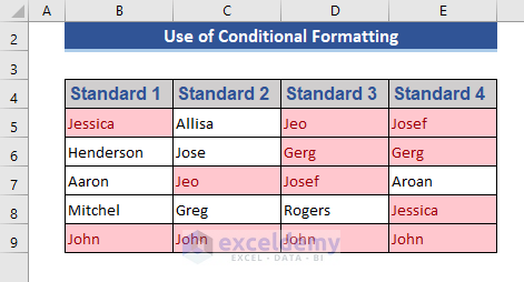
Here, the duplicate cells are colored red after comparing the given 4 columns.
Read More: How to Compare 3 Columns for Matches in Excel
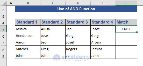
Method 2 – Using the AND Function
The AND function is one of the logical functions. It is used to determine if all conditions in a test are TRUE or not. The AND function returns TRUE if all its arguments evaluate TRUE and returns FALSE if one or more arguments evaluate FALSE.
Syntax:
AND(logical1, [logical2], …)
Argument:
logical1 – The first condition that we want to test can evaluate as either TRUE or FALSE.
logical2, … – Additional conditions that you want to test that can evaluate to either TRUE or FALSE, up to a maximum of 255 conditions.
2.1 AND Function with Cells
Steps:
- Add a column and name it ‘Match’ in the dataset.
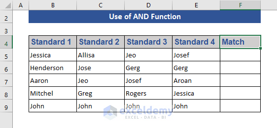
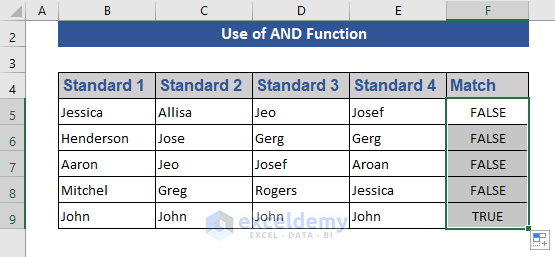
- Enter the AND function and compare each of the 4 column cells individually. The formula is:
=AND(B5=C5,C5=D5,D5=E5)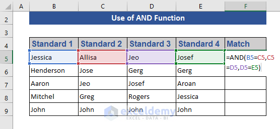
- Press Enter.
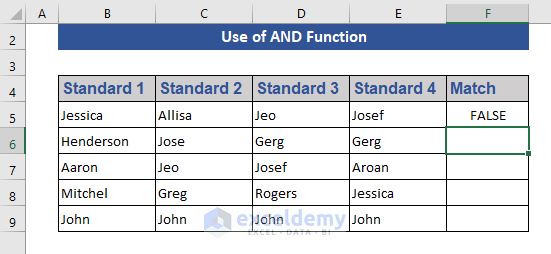
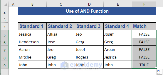
- Drag the Fill Handle icon to the end of the column.
2.2 AND Function with Range
Steps:
- Modify the AND function. Use the following formula:
=AND(B5=C5:E5)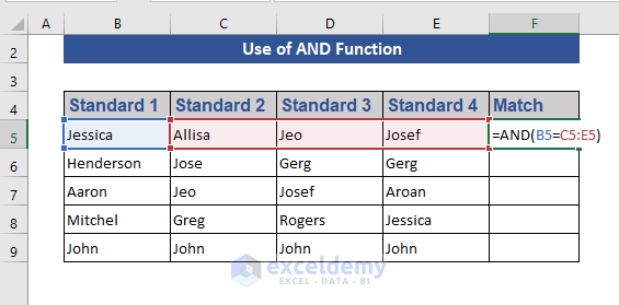
- Press Ctrl+Shift+Enter.
- Drag the Fill Handle icon to the end of the column.
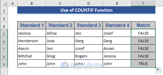
Method 3 – Using the COUNTIF Function
Syntax:
COUNTIF(range, criteria)
Argument:
range –This is the group of cells we will count. The range can contain numbers, arrays, a named range, or references that contain numbers. Blank and text values are ignored.
criteria – It may be a number, expression, cell reference, or text string that determines which cells will be counted. COUNTIF uses only a single criterion.
a)
Steps:
- Go to cell F5.
- Enter the COUNTIF function. The formula is:
=COUNTIF(B5:E5,B5)=4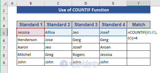
- Press Enter.
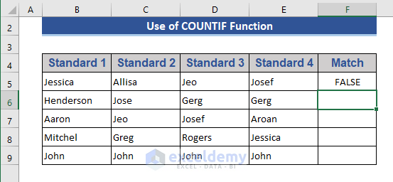
- Pull the Fill Handle to cell F9.
b)
Steps:
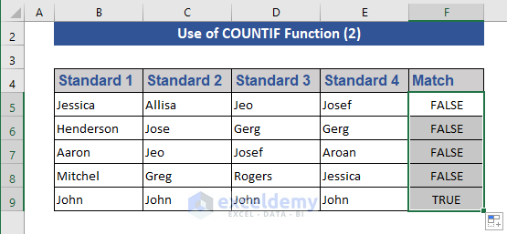
- Modify the COUNTIF function in cell F5. The formula is:
=COUNTIF(B5:E5,"<>"&B5)=0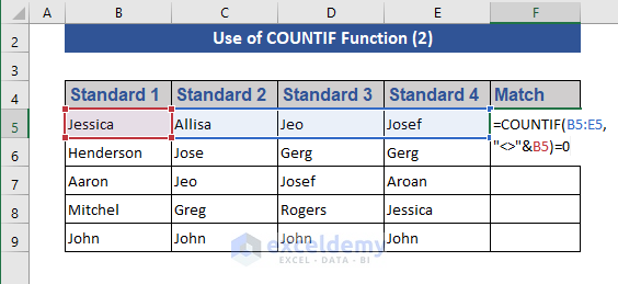
- Press Enter.
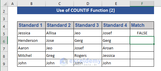
- Pull the Fill Handle icon to the last cell.
Method 4 – Inserting the VLOOKUP Function
Syntax:
VLOOKUP (lookup_value, table_array, col_index_num, [range_lookup])
Argument:
lookup_value – The value we want to look up. It must be in the first column of the range of cells we specify in the table_array argument. Lookup_value can be a value or a reference to a cell.
table_array – The range of cells in which the VLOOKUP will search for the lookup_value and the return value. We can use a named range or a table, and you can use names in the argument instead of cell references.
col_index_num – The column number (starting with 1 for the left-most column of table_array) that contains the return value.
range_lookup – A logical value that specifies whether we want VLOOKUP to find an approximate or an exact match.
Steps:
- Set a criteria option in the dataset.
- Select John as the criteria.
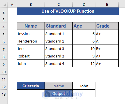
- Enter the VLOOKUP function in cell D13.
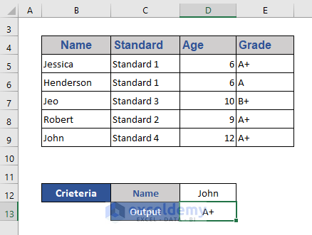
- Search cell D12 from the range and get values of the 4th column, Grade. The formula is:
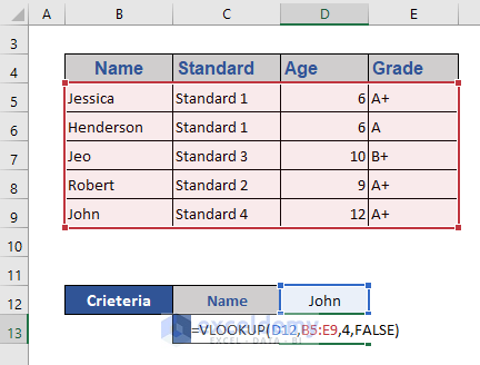
- Press Enter.
Method 5 – Combining MATCH & INDEX Functions
Syntax:
INDEX(array, row_num, [column_num])
Argument:
array – A range of cells or an array constant.
If an array contains only one row or column, the corresponding row_num or column_num argument is optional.
If the array has more than one row and more than one column and only row_num or column_num is used, INDEX returns an array containing the entire row or column.
row_num – This selects the row in the array from which to return a value. If row_num is omitted, column_num is required.
column_num – This selects the column in the array from which to return a value. If column_num is omitted, row_num is required.
The MATCH function searches for a specified item in a range of cells and then returns the relative position of that item in the range.
Syntax:
MATCH(lookup_value, lookup_array, [match_type])
Argument:
lookup_value – This is the value we want to match in lookup_array. The lookup_value argument can be a value (number, text, or logical value) or a cell reference to a number, text, or logical value.
lookup_array – The range of cells where we search.
match_type – The number -1, 0, or 1. The match_type argument specifies how Excel matches lookup_value with values in lookup_array. The default value for this argument is 1.
Steps:
- Set Jeo as the criteria in cell D12.
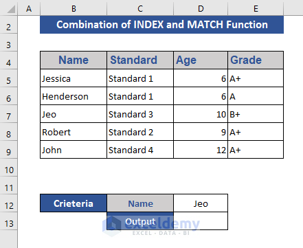
- Enter the following formula in cell D13:
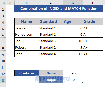
=INDEX(D5:D9,MATCH(D12,B5:B9,0))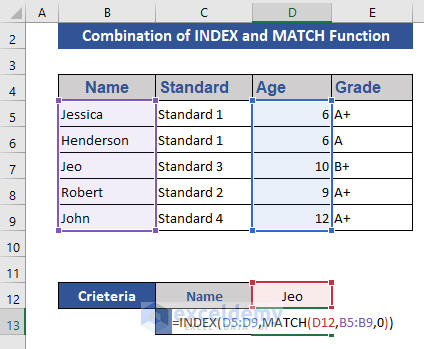
- Press Enter.
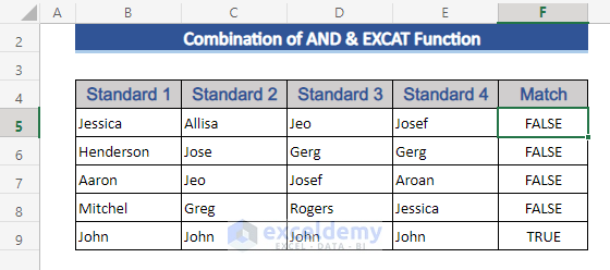
Method 6 – Merging AND & EXACT Functions
Syntax:
EXACT(text1, text2)
Arguments:
text1 – The first text string.
text2 – The second text string.
Steps:
- Go to cell F5.
- Enter the following formula:
=AND(EXACT(B5:E5,B5))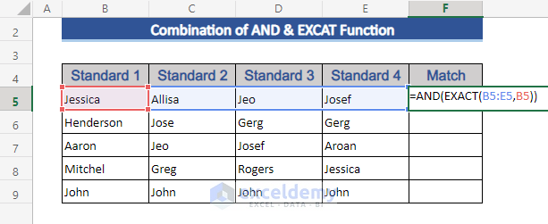
- Press Enter.
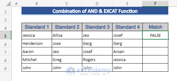
- Pull the Fill Handle icon to the last column.
Download the Practice Workbook
Download this workbook to practice.
<< Go Back to Columns | Compare | Learn Excel
Get FREE Advanced Excel Exercises with Solutions!
