Microsoft Excel offers several options for comparing columns, but most of them are for searching in one column only. This article will demonstrate several techniques to compare two columns and return common values.
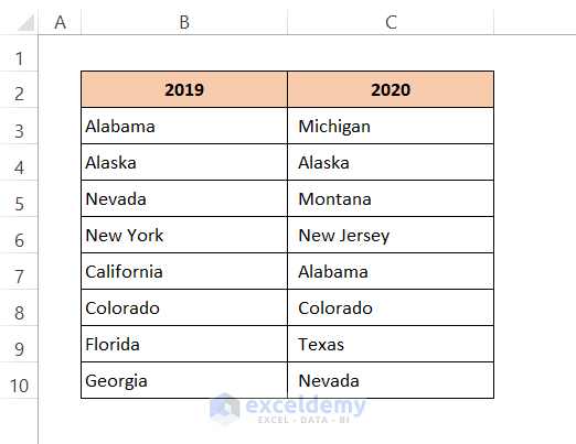
In our sample dataset, we have the participants of a basketball tournament in two consecutive years. Some States are common to both years. Let’s compare them and return common values using 3 quick tricks in Excel.
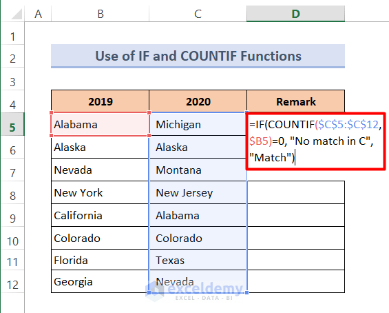
Trick 1 – Using IF + COUNTIF
Steps:
- In cell D5 enter the formula below:
=IF(COUNTIF($C$5:$C$12, $B5)=0, "No match in C", "Match")- Press Enter.
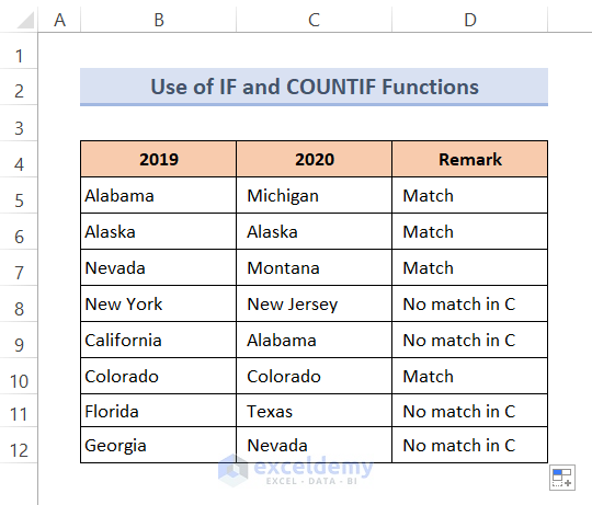
- Use the Fill Handle tool to copy the formula to the other cells.
Our desired output is returned.
Formula Breakdown:
➥ COUNTIF($C$5:$C$12, $B5)=0
The COUNTIF function will check whether the value of Cell B5 through the range C5:C12 is equal or not. If equal then it will return 1 otherwise 0. It returns:
FALSE
➥ IF(COUNTIF($C$5:$C$12, $B5)=0, “No match in C”, “Match”)
The IF function will show ‘No match in C’ for FALSE and ‘Match’ for TRUE. It returns:
Match
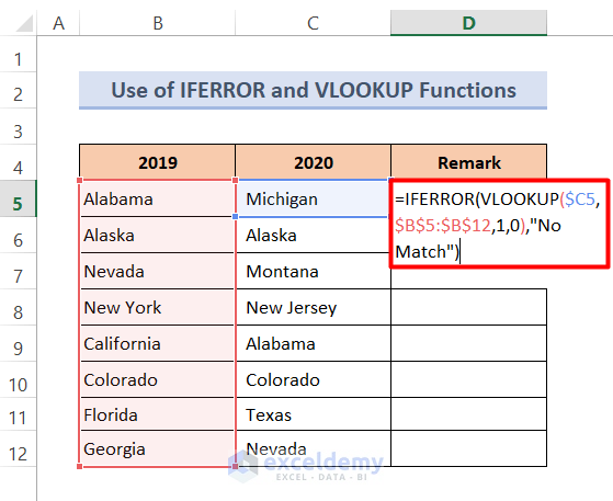
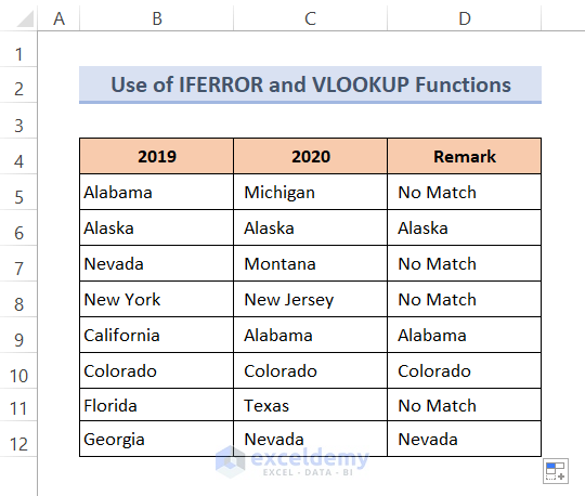
Trick 2 – Using IFERROR + VLOOKUP
Let’s check whether the values of Column D have a match in Column C or not using the IFERROR and VLOOKUP Functions. If a match is found then it will return the State name otherwise it will display “No Match“. The IFERROR function is used to trap and manage errors in formulas and calculations. The VLOOKUP function is used to look up a value in the leftmost column of a table and returns the corresponding value from a column to the right.
Steps:
- Enter the formula below in Cell D5:
=IFERROR(VLOOKUP($C5,$B$5:$B$12,1,0),"No Match")- Press Enter and use the Fill Handle to copy the formula to the rest of the cells in the column.
Here’s our output:
Formula Breakdown:
➥ VLOOKUP($C5,$B$5:$B$12,1,0)
The VLOOKUP function will check cell C5 through the range B5:B12. If it finds a common value then it will show that value otherwise it will display #N/A. For cell C5 it returns:
#N/A
➥ IFERROR(VLOOKUP($C5,$B$5:$B$12,1,0),”No Match”)
The IFERROR function will show “No Match” for #N/A results, and the other output will remain the same. For Cell C5 it returns:
“No Match”
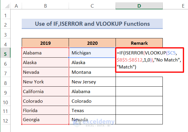
Trick 3 – Using IF + ISERROR + VLOOKUP
Steps:
- In cell D5 enter the formula below:
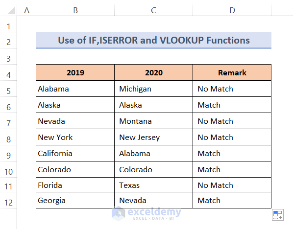
=IF(ISERROR(VLOOKUP($C12,$B$5:$B$12,1,0)),"No Match","Match")- Press Enter and use the AutoFill option to return all the results.
The cells with common values are identified.
Formula Breakdown:
➥ VLOOKUP($C5,$B$5:$B$12,1,0)
The VLOOKUP function will check cell C5 through the range B5:B12. If it finds a common value then it will display that value otherwise it will show #N/A. For cell C5 it returns:
#N/A
➥ ISERROR(VLOOKUP($C5,$B$5:$B$12,1,0))
The ISERROR function will show TRUE for #N/A and FALSE for other output. It returns:
TRUE
➥ IF(ISERROR(VLOOKUP($C5,$B$5:$B$12,1,0)),”No Match”,”Match”)
The IF function will return “No Match” for TRUE and “Match” for FALSE. It returns:
“No Match”
Now let’s examine some ways of highlighting the common values as opposed to returning them.
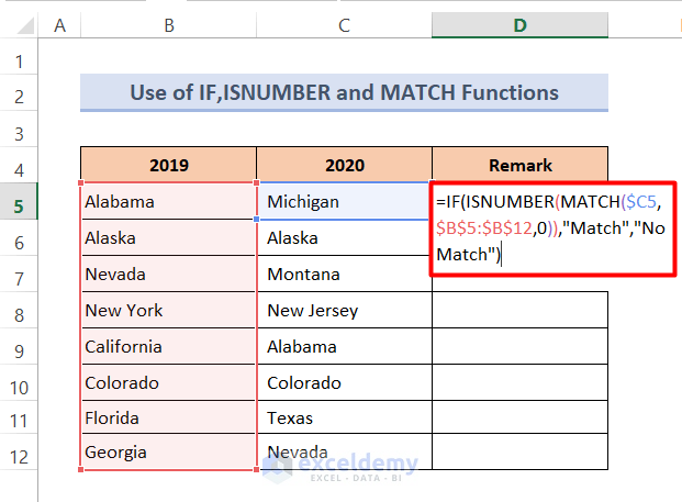
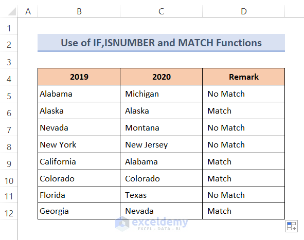
Method 1 – Using IF, ISNUMBER and MATCH Functions
The ISNUMBER function will return TRUE if a cell contains a number, and FALSE if not. The MATCH function searches for a specified item in a range of cells and then returns the relative position of that item in the range.
Steps:
- Enter the formula below in Cell D5:
=IF(ISNUMBER(MATCH($C5,$B$5:$B$12,0)),"Match","No Match")- Press Enter.
- Use the Fill Handle icon to copy the formula to the rest of the cells.
The result is as follows:
Formula Breakdown:
➥ MATCH($C5,$B$5:$B$12,0)
The MATCH function will return the relative position number of matched values in the range B5:B12. If doesn’t match then it will show #N/A. It returns:
#N/A
➥ ISNUMBER(MATCH($C5,$B$5:$B$12,0))
The ISNUMBER function will show TRUE for numbers and FALSE for errors. It returns:
FALSE
➥ IF(ISNUMBER(MATCH($C5,$B$5:$B$12,0)),”Match”,”No Match”)
The IF function will show “Match” for TRUE and “No Match” for FALSE. It returns:
“No Match”
Read More: Excel formula to compare two columns and return a value
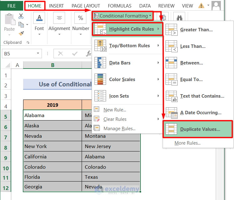
Method 2 – Using Conditional Formatting with Built-in Rules
Let’s highlight all the common values with a selected color.
Steps:
- Select the data range B5:C12.
- Click Home > Conditional Formatting > Highlight Cells Rules > Duplicate Values.
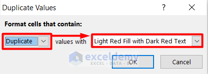
A dialog box will open up.
- Select the Duplicate option and desired color from the Format cells that contain box.
- Click OK.
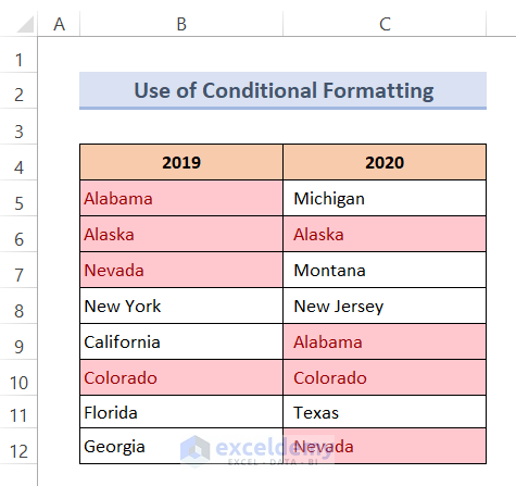
All the common values are highlighted with the selected color.
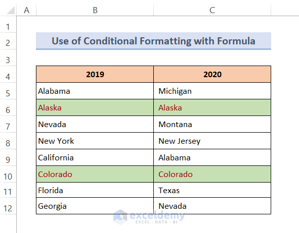
Method 3 – Using Conditional Formatting with New Rules to Return Common Values (Same Row)
Now let’s find common values in the same row only.
Steps:
- Select the data range B5:C12.
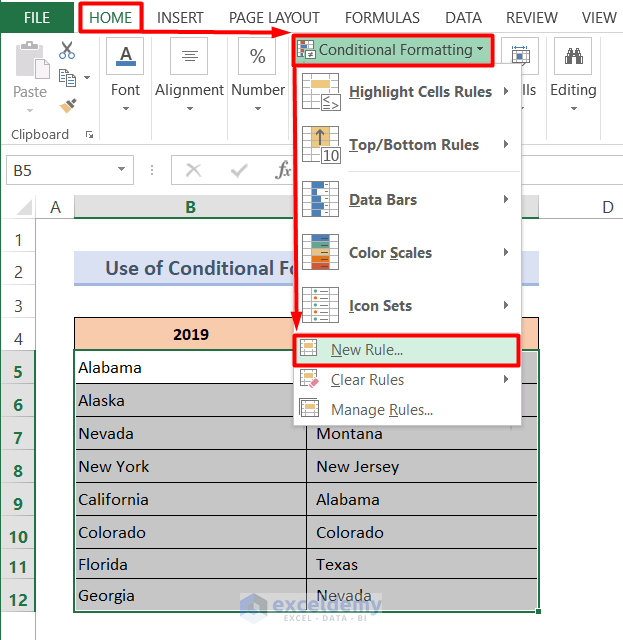
- Click Home > Conditional Formatting > New Rule.
A dialog box will appear.
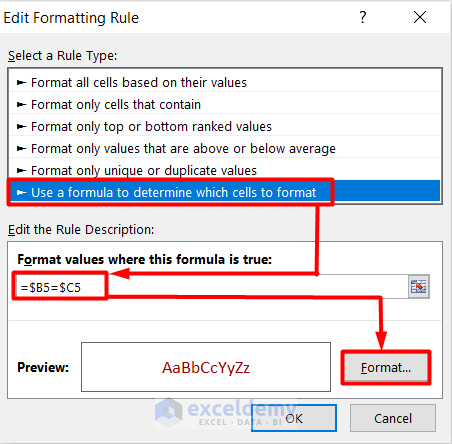
- Click Use a formula to determine which cells to format from the Select a Rule Type box.
- Enter the formula below in the Format values where this formula is true box.
=$B5=$C5⏩Then click Format.
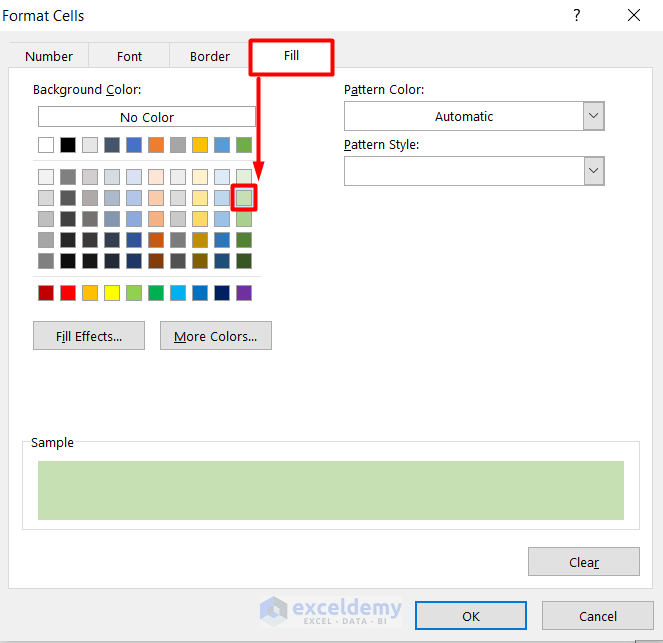
Then ‘Format Cells’ dialog box will appear.
- Choose your desired color from the Fill option. Here, a light green color.
- Click OK to return to the previous dialog box.
- Click OK.
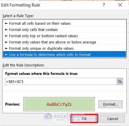
All the common values in the same row are now highlighted with the selected color.
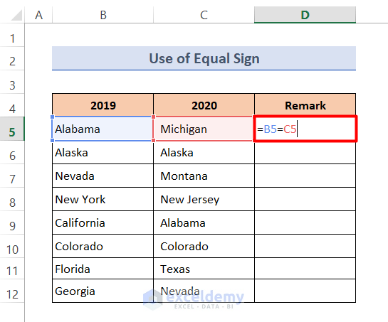
Method 4 – Applying Boolean Logic to Compare and Return Common Values from the Same Row
We can find common values in the same row using the Equal Sign(=) too. If the same values are found then it will show TRUE otherwise FALSE. To display the output we add a new column named ‘Remark’.
Steps:
- Enter the formula below in cell D5:
=B5=C5- Press Enter to return the output.
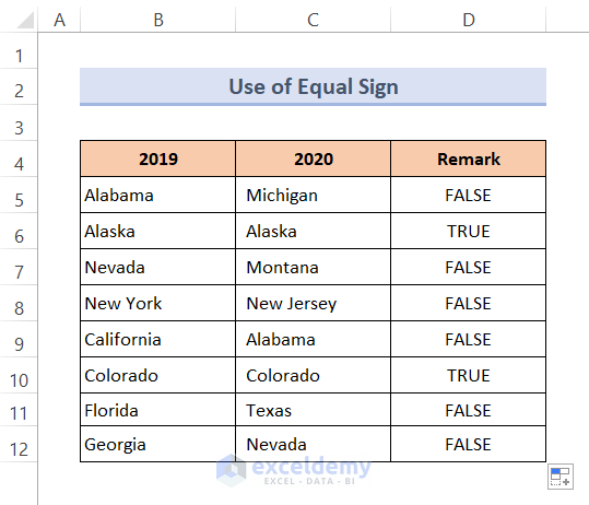
- Double-click the Fill Handle icon to copy the formula.
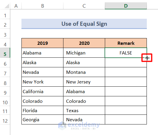
The desired output is returned.
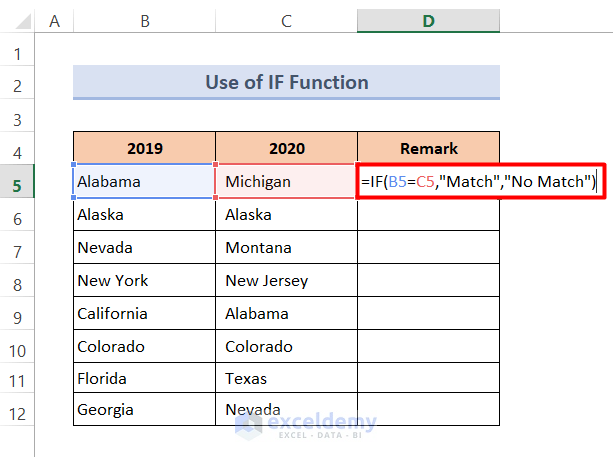
Method 5 – Using the IF Function for Common Values in the Same Row
Here, the IF function will show ‘Match’ in the case of common values in the same row, and ‘No Match’ if not.
Steps:
- In cell D5, enter the formula below:
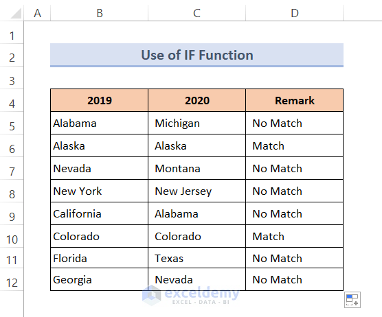
=IF(B5=C5,"Match","No Match")- Press Enter.
- Use the Fill Handle tool to copy the formula.
The result is as follows:
Download Practice Workbook
<< Go Back to Columns | Compare | Learn Excel
Get FREE Advanced Excel Exercises with Solutions!
