Excel Formula to Compare and Return Value from Two Columns

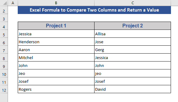
We’ll use a simple dataset of employees assigned to two projects for a few of the methods.

Method 1 – Combining Excel IF and EXACT Functions to Compare Two Columns and Return a Value

Syntax:

IF(logical_test, value_if_true, [value_if_false])

Argument:

logical_test – The desired condition we want to test.

value_if_true – The value we want to return if the result of logical_test is TRUE.

value_if_false – The value will return if the result of logical_test is FALSE.

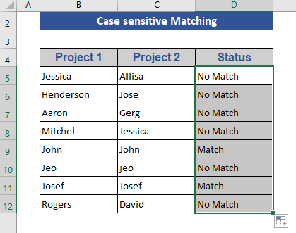
Case 1.1 – Case-Insensitive Search

This approach is not case-sensitive, which means Jeo and jeo are considered the same.

Steps:

• Go to Cell D5.
• Insert the following formula:

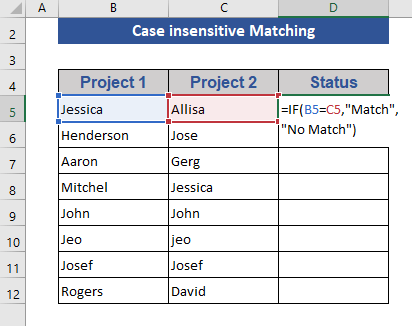
• Press Enter.

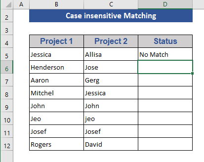
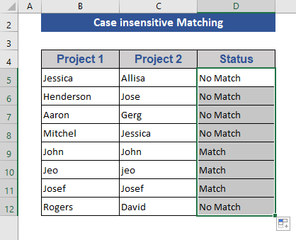
• Pull the Fill Handle icon down.

Case 1.2 – Case-sensitive Approach

The EXACT function compares two text strings and returns TRUE if they are the same. EXACT is case-sensitive but ignores formatting differences.

Syntax:

EXACT(text1, text2)

Arguments:

text1 – It is the first text string.

text2 – It is the second text string.

Steps:

• Go to Cell D5.
• Modify the IF function with the EXACT function:

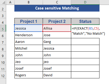
• Press the Enter button.

• Drag the Fill Handle icon down.

Read More: Excel formula to compare two columns and return a value

Method 2 – Merging Excel IF, ISNA, and MATCH Functions to Return Mismatched Items from the Second Column

Steps:

• Go to cell D5 and insert the following formula:

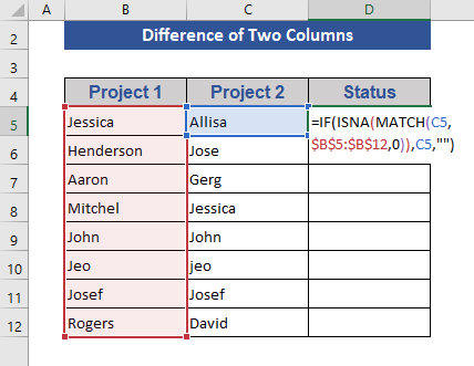
• Press Enter.

• Pull the Fill Handle icon down.

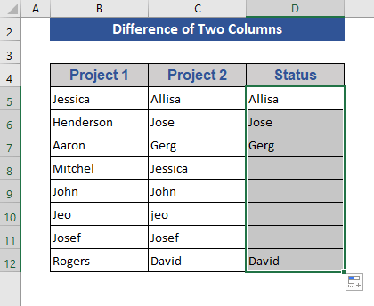
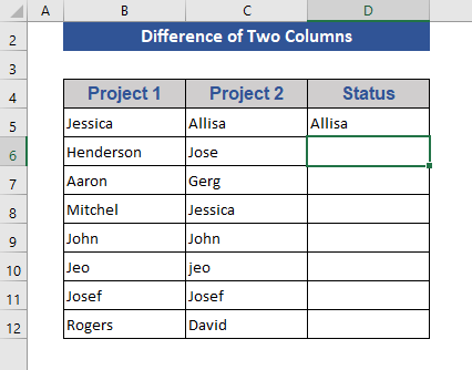
In the status box, we see those names that are present only in Project 2 but not in Project 1.

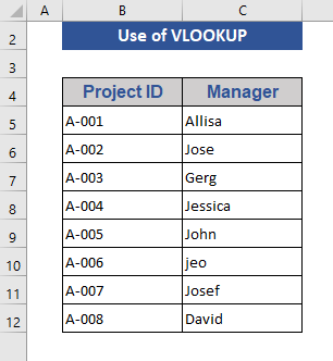
Method 3 – Inserting a VLOOKUP Function to Compare and Return Values from Two Columns

We modified the dataset to include Project IDs and employees assigned to each one.

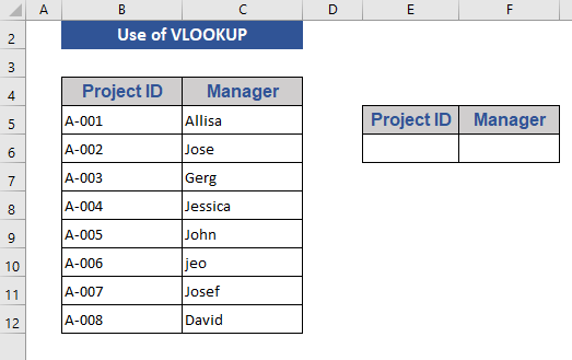
Steps:

• Add two boxes for Project ID and Manager.
• Input the Project ID manually.

• We put Project ID as A-003.

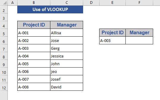
• Go to cell F6.
• Use this formula:

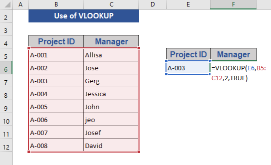
• Press Enter.

We get the Manager’s name by inputting the Project ID.

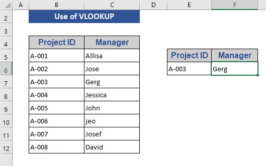
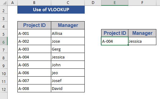
• Change the Project ID and press Enter to see the changes.

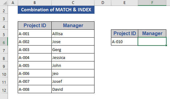
Method 4 – Joining INDEX and MATCH Functions to Compare Two Columns and Return a Value

Steps:

• We put A-007 as the Project ID in Cell E6.

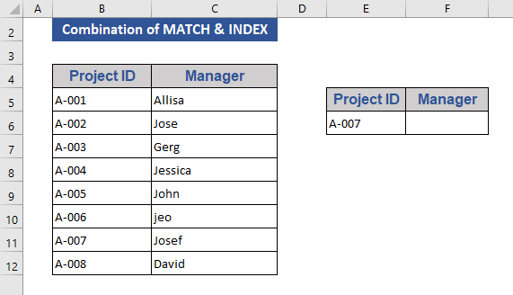
• Use this formula in the result cell:

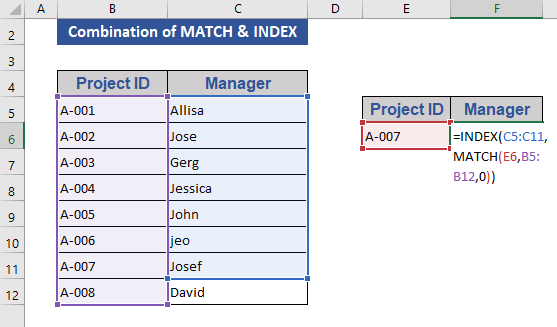
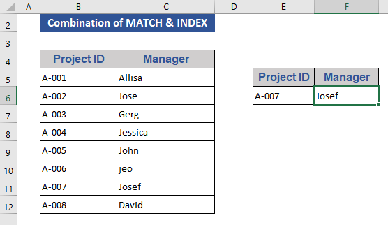
• Press Enter.

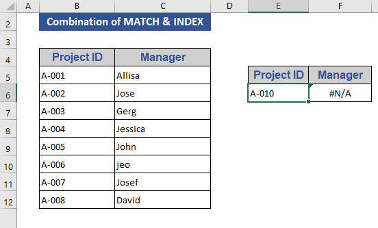
• If we input A-010 and press Enter, the result is #N/A.

• Modify the formula in the result cell to the following:

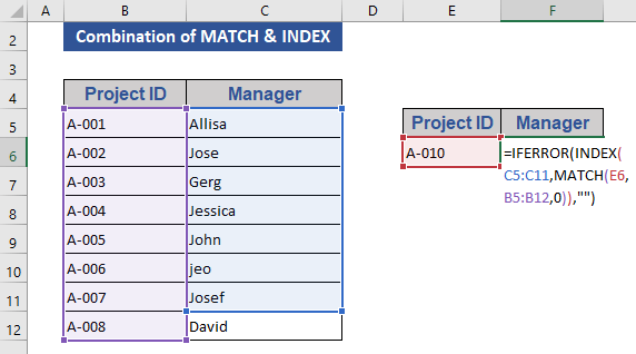
• Press Enter.

If the reference is not found, the result will be blank.

Formula Breakdown:

• MATCH(E6,B5:B12,0)

This function searches for a match of Cell E6 in the range B5 to B12.

Output: 7

• INDEX(C5:C11,MATCH(E6,B5:B12,0))

This function searches the output of the MATCH function on the range C5 to C11.

Output: Josef

• IFERROR(INDEX(C5:C11,MATCH(E6,B5:B12,0)),””)

This will return the value of INDEX if the value is valid, otherwise, the cell will show blank.

Output: Josef

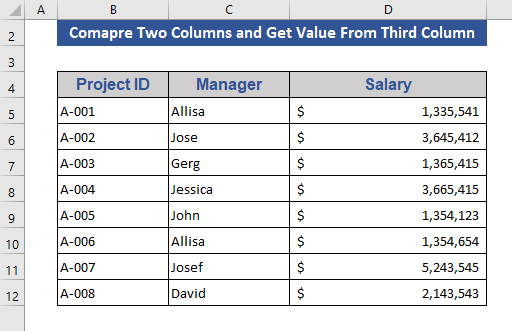
Method 5 – Comparing Two Columns and Return a Value from the Third Column

We will compare two columns and get results from the third column. We entered a third column for the results.

Steps:

• Use Project ID and Manager as references to compare and get the output from Salary.

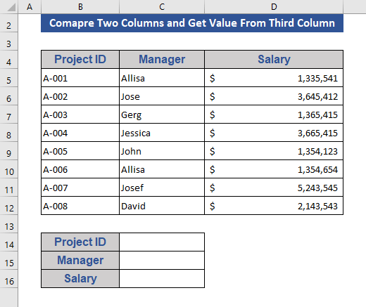
• Manually input the reference values.

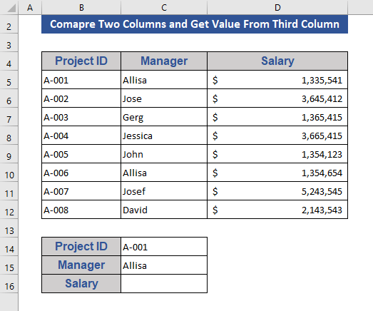
• Use this formula in Cell C16:

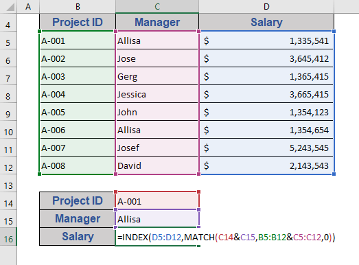
• Press Ctrl + Shift + Enter as it is an array function.

Download the Practice Workbook

<< Go Back to Columns | Compare | Learn Excel