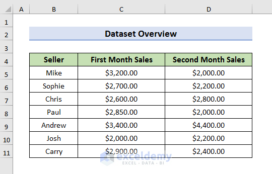
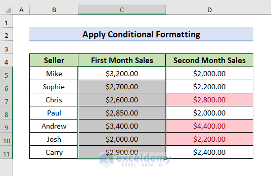
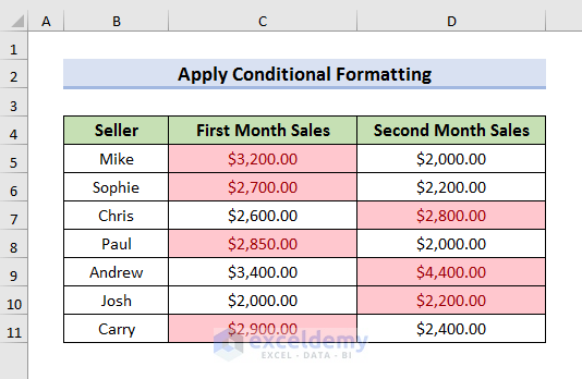
The sample dataset contains information about the sales amount of some salespeople for two months. We will compare the sales of the first month with the sales of the second month and highlight the greater value.
Method 1 – Using Excel Conditional Formatting to Compare Two Columns and Highlight the Greater Value
STEPS:
- Select cells from Column D.
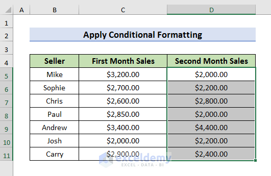
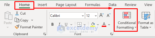
- Go to the Home tab and select Conditional Formatting. A drop-down menu will appear.

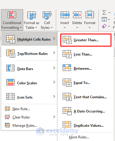
- Select Highlight Cells Rules and then select Greater Than. It will open a Greater Than window.

- Enter the formula below in the Greater Than window.
=C5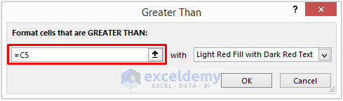
- Click OK.
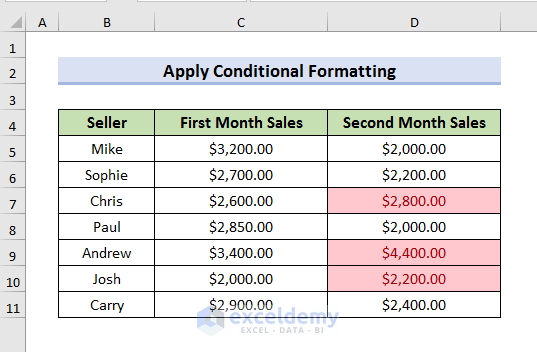
- The cells that contain greater values compared to Column C are highlighted.
- Select the cells of Column C.
- Go to the Home tab and select Conditional Formatting.
- Select Highlight Cells Rules and then select Greater Than from the drop-down menu.
- Enter the formula below in the Greater Than window.
=D5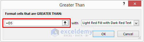
- Click OK.
- The cells that contain greater values compared to Column D are highlighted.
Read More: Excel formula to compare two columns and return a value
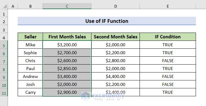
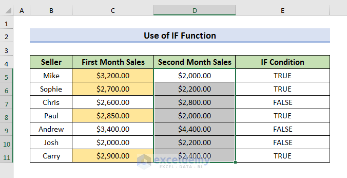
Method 2 – Use IF Function to Compare Two Columns and Highlight the Higher Value in Excel
STEPS:
- Create an extra column in your dataset. Column E is our new column.
- Select Cell E5 and enter the formula:
=IF(C5>D5,"TRUE","FALSE")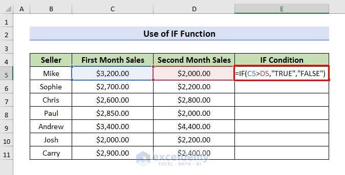
- Hit Enter to see the result.
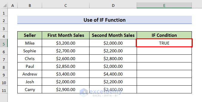
The IF Function is checking whether Cell C5 is greater than Cell D5. If it is true, then it displays TRUE in the output column, and if Cell D5 is greater than Cell C5, then it shows False.
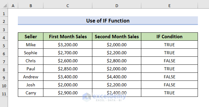
- Use the Fill Handle to see results of each salesperson.
STEPS:
- To instead highlight the greater value, select the cells of Column C. We have selected Cell B5 to Cell B11.
- Go to the Home tab and select Conditional Formatting. A drop-down menu will appear.

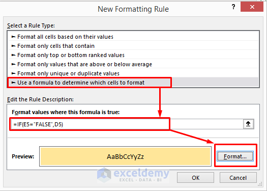
- Select New Rule from the drop-down menu. The New Formatting Rule window will occur.

- Select Use a formula to determine which cells to format from the Select a Rule Type field.
- Enter the formula below in the Format values where this formula is true field:
=IF(E5="TRUE",C5)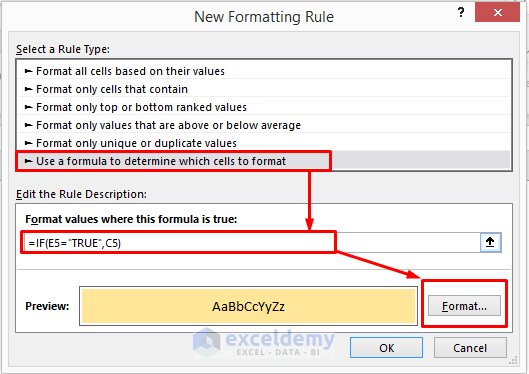
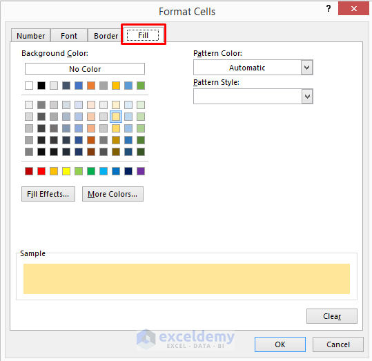
- Click Format.
- Select Fill from the Format Cells window and choose a color to highlight the cells.
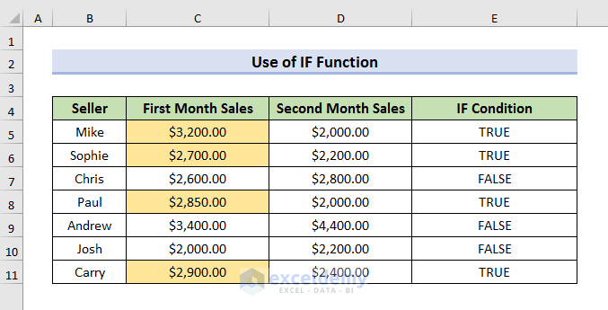
- Click OK to proceed and click OK in the New Formatting Rule window.
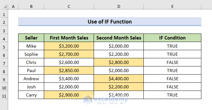
- After clicking OK, you will see results like below.
- Select the cells of Column D.
- Go to the Home tab and select Conditional Formatting.
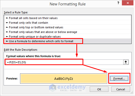
- Select the New Rule. The New Formatting Rule window will appear.
- Select Use a formula to determine which cells to format from the Select a Rule Type field.
- Enter the below formula in the Format values where this formula is true field:
=IF(E5="TRUE",D5)- Select Format and choose a color then and click OK.
- Click OK in the New Formatting Rule window to return the results as below.
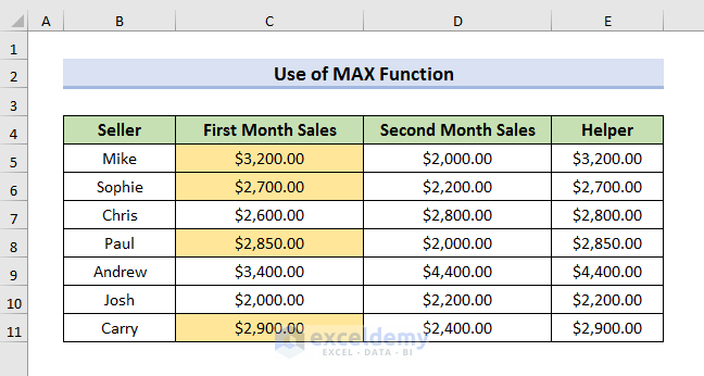
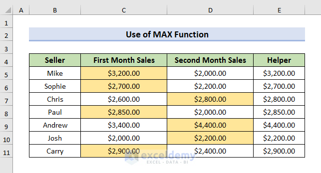
Method 3 – Compare Two Columns and Highlight the Greater Value with MAX Functio
STEPS:
- Create an extra column at the beginning. Column E is our extra column.
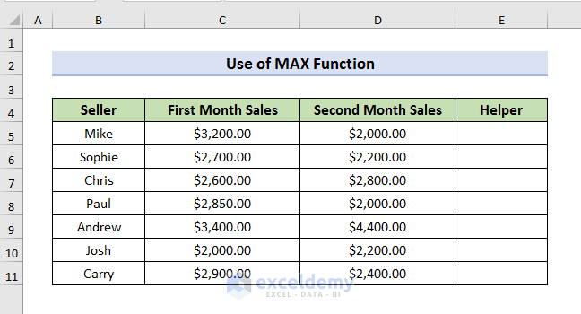
- Select Cell E5 and enter the formula:
=MAX(C5,D5)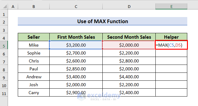
- Hit Enter to see the result.
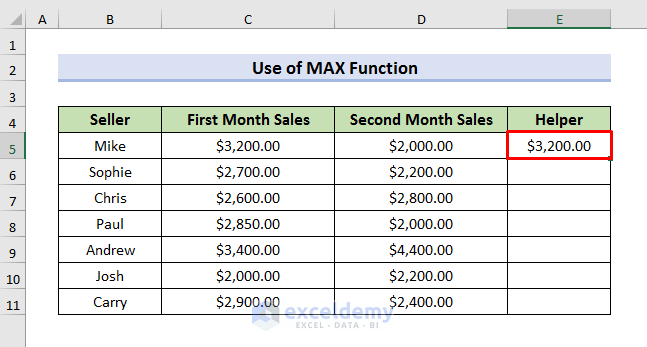
Here, the MAX Function is comparing the value between Cell C5 and Cell D5. It then shows the greater value in the Helper column.
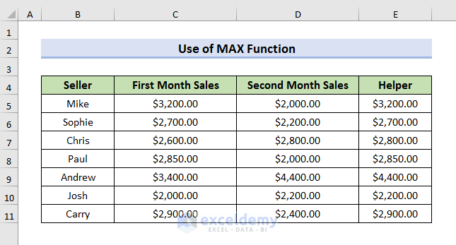
- Use the Fill Handle to see all the results.
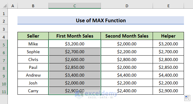
To highlight the greater value, we will use conditional formatting.
STEPS:
- Select the values of Column C.
- Go to the Home tab and select Conditional Formatting. A drop-down menu will appear.

- Select New Rule from the drop-down menu.

- The New Formatting Rule window will appear.
- Select Use a formula to determine which cells to format from the Select a Rule Type field.
- Enter the below formula in the Format values where this formula is true field:
=IF(C5=E5,C5)- Select Format.
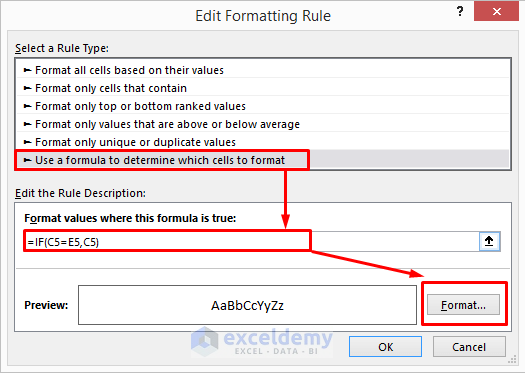
- After selecting Format, the Format Cells window will appear.
- Select Fill and choose a color to highlight the cells.
- Click OK to proceed.
- Click OK in the New Formatting Rule window.

- The results are returned as below.
- To highlight the greater values of Column D, select Cell D5 to Cell D11.
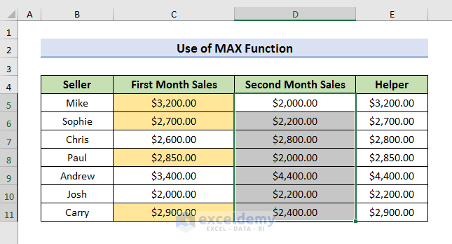
- Go to the Home tab and select Conditional Formatting.
- Select the New Rule from there. It will open the New Formatting Rule window.
- Select Use a formula to determine which cells to format from the Select a Rule Type field.
- Enter the formula in the Format values where this formula is true field:
=IF(D5=E5,D5)- Select Format to choose a color and click OK to proceed.
- Click OK in the New Formatting Rule window.
- The results are returned as below.
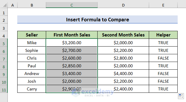
Method 4 – Insert Formula to Compare Two Columns in Excel and Highlight the Greater Value
STEPS:
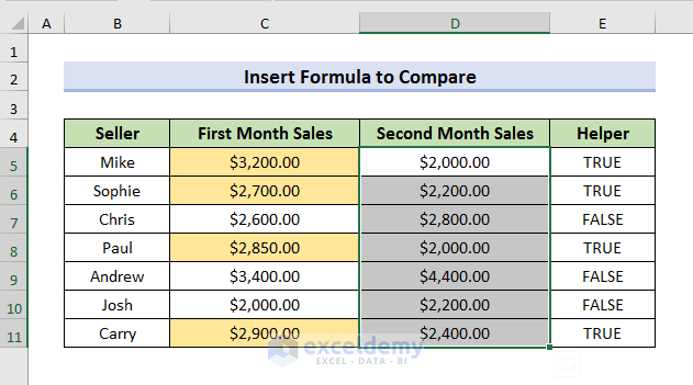
- Insert a helper column and type the formula:
=C5>D5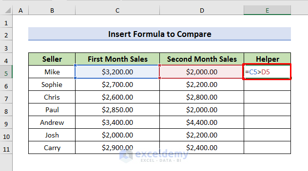
- Hit Enter to see the result.
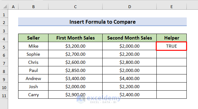
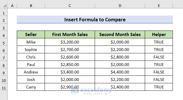
Here, the formula checks whether the value of Cell C5 is greater than Cell D5. If Cell C5 is greater than Cell D5, then it will display TRUE in the output. Otherwise, it will show False.
- Use the Fill Handle to see results of all rows.
You can highlight the greater values with conditional formatting.
STEPS:
- Select the values of Column C.
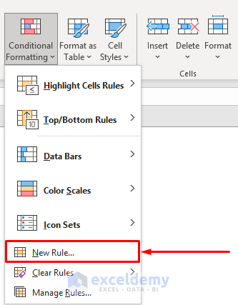
- Go to the Home tab and select Conditional Formatting.

- A drop-down menu will appear.
- Select New Rule from there. It will open the New Formatting Rule window.
- Select Use a formula to determine which cells to format from the Select a Rule Type field.
- Enter the below formula in the Format values where this formula is true field:
=IF(C5>D5,C5)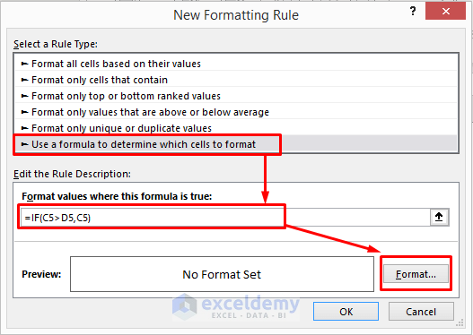
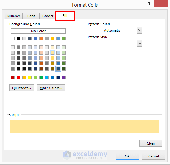
- It will open the Format Cells window.
- Select Fill from the Format Cells window and choose a color to highlight the cells.
- Click OK to proceed.
- Click OK in the New Formatting Rule window.
- The greater values of Column C will be highlighted.
- Select the values of Column D to highlight.
- Follow the same steps to open the New Formatting Rules field.
- Select Use a formula to determine which cells to format from the Select a Rule Type field.
- Enter the below formula in the Format values where this formula is true field:
=IF(D5>C5,D5)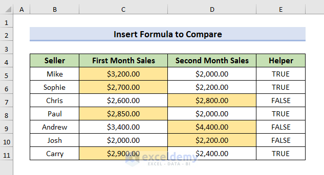
- Select Format to choose the color and click OK.
- Click OK in the New Formatting Rule window.
- The results are returned as below.
Download Practice Book
Download the practice book here.
<< Go Back to Columns | Compare | Learn Excel
Get FREE Advanced Excel Exercises with Solutions!
