Method 1 – Using a VBA Macro to Compare Two Columns and Highlight the Differences in Excel
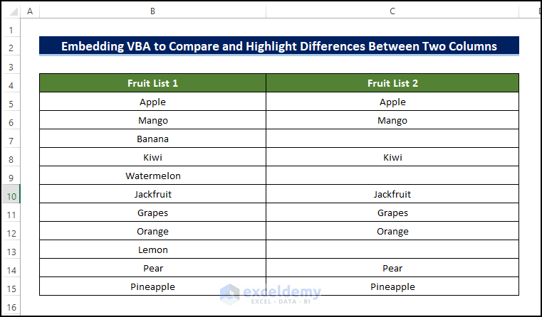
This is the sample dataset.
Steps:
- Press Alt + F11 or go to Developer -> Visual Basic to open the Visual Basic Editor.

- Click Insert -> Module.
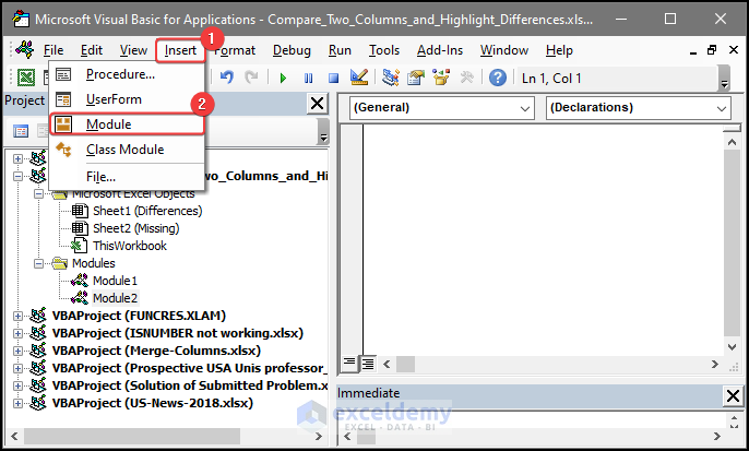
- Copy the following code into the code window.
Sub HighlightColumnDifferences()
Dim Rg As Range
Dim Ws As Worksheet
Dim FI As Integer
 On Error Resume Next
 SRC:
 Set Rg = Application.InputBox("Select Two Columns:", "Excel", , , , , , 8)
 If Rg Is Nothing Then Exit Sub
 If Rg.Columns.Count <> 2 Then
     MsgBox "Please Select Two Columns"
     GoTo SRC
 End If
Set Ws = Rg.Worksheet
For FI = 1 To Rg.Rows.Count
     If Not StrComp(Rg.Cells(FI, 1), Rg.Cells(FI, 2), vbBinaryCompare) = 0 Then
        Ws.Range(Rg.Cells(FI, 1), Rg.Cells(FI, 2)).Interior.ColorIndex = 8 'you can change the color index as you like.
End If
 Next FI
 End Sub
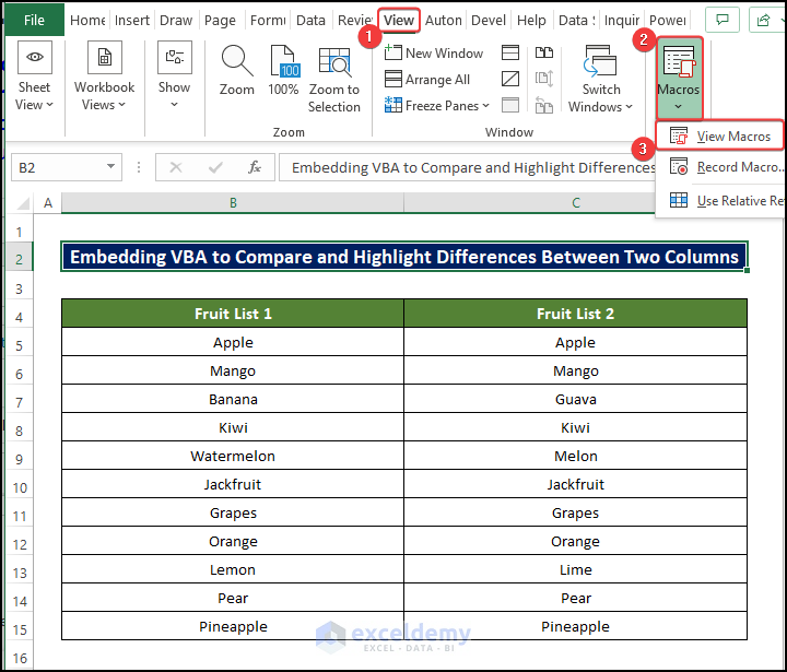
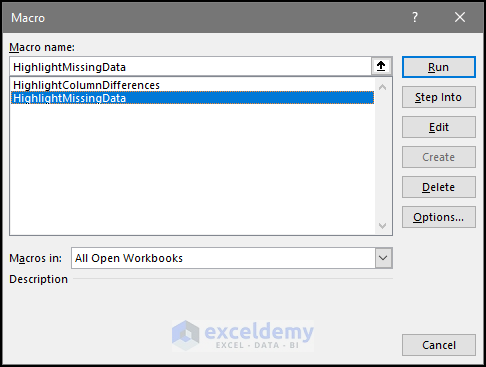
- Go to View> Macros>View Macros.
- In the dialog box, select HighlightColumnDfferences and click Run.
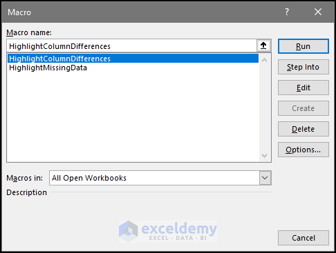
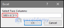
- In the new dialog box, enter the location of the two columns: B5:C15
- Click OK.
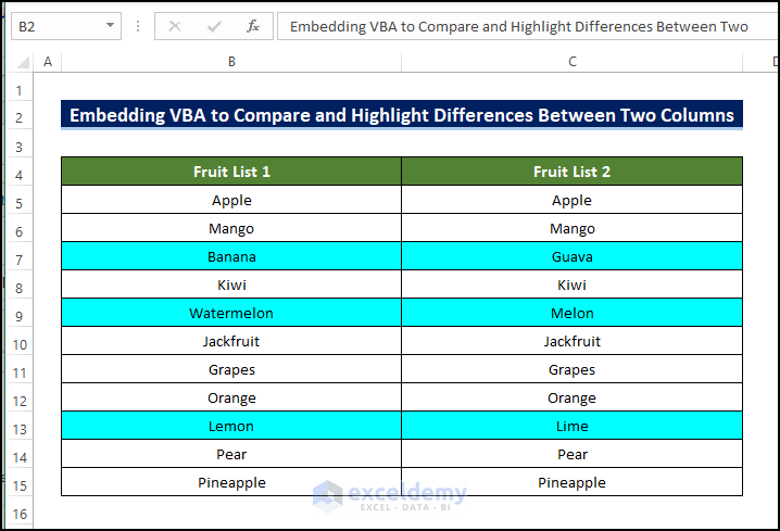
This is the output.
Read More: Excel formula to compare two columns and return a value
Method 2 – Using a VBA Macro to Compare Two Columns and Highlight Differences in Missing Data in Excel
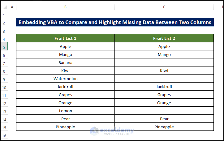
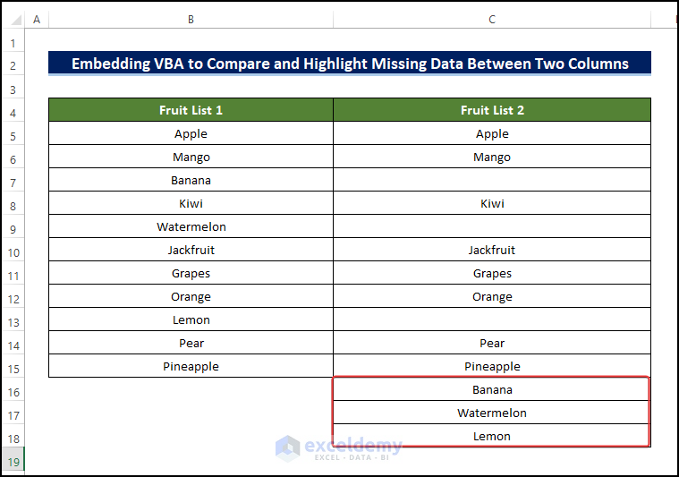
In the dataset below, Fruit List 2 has missing data:
Steps:
- Open the Visual Basic Editor in the Developer tab and insert a Module.
- Enter the following code.
Sub HighlightMissingData()
Dim Rg, RgC1, RgC2, FRg1, FRg2 As Range
Dim IntR, IntSR, IntER, IntSC, IntEC As Integer
Dim Ws As Worksheet
On Error Resume Next
SRC:
 Set Rg = Application.InputBox("Select Two Columns:", "Excel", , , , , , 8)
 If Rg Is Nothing Then Exit Sub
If Rg.Columns.Count <> 2 Then
     MsgBox "Please Select Two Columns as a Range"
    GoTo SRC
 End If
Set Ws = Rg.Worksheet
IntSC = Rg.Column
IntEC = Rg.Columns.Count + IntSC - 1
IntSR = Rg.Row
IntER = Rg.Rows.Count + IntSR - 1
   Set Rg = Rg.Columns
Set RgC1 = Ws.Range(Ws.Cells(IntSR, IntSC), Ws.Cells(IntER, IntSC))
Set RgC2 = Ws.Range(Ws.Cells(IntSR, IntEC), Ws.Cells(IntER, IntEC))
IntR = 1
 For Each FRg In RgC1
    If WorksheetFunction.CountIf(RgC2, FRg.Value) = 0 Then
        Ws.Cells(IntER, IntEC).Offset(IntR) = FRg
         IntR = IntR + 1
    End If
 Next
IntR = 1
For Each FRg In RgC2
    If WorksheetFunction.CountIf(RgC1, FRg) = 0 Then
        Ws.Cells(IntER, IntSC).Offset(IntR) = FRg
         IntR = IntR + 1
    End If
 Next
End Sub- Go to View> Macros>View Macros.
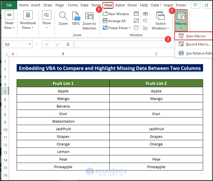
- Select HighlightMissingData and click Run.
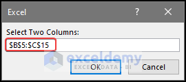
- In the new dialog box, enter B5:C15.
- Click OK.
This is the output.
Download Practice Template
Download the free practice Excel template.
<< Go Back to Columns | Compare | Learn Excel
Get FREE Advanced Excel Exercises with Solutions!
