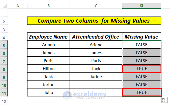
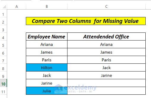
The sample dataset showcases Employee Name and Attended Office. Find the names of employees who didn’t attend the office.
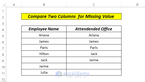
Method 1 – Joining the VLOOKUP and the ISERROR Functions to Compare Two Columns in Excel and find Missing Values
Steps:
- Select D5 and enter the following formula.
=ISERROR(VLOOKUP(B5,$C$5:$C$11,1,0))
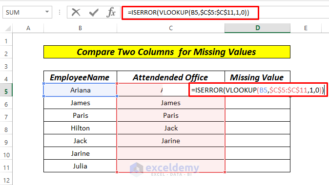
- Press ENTER.
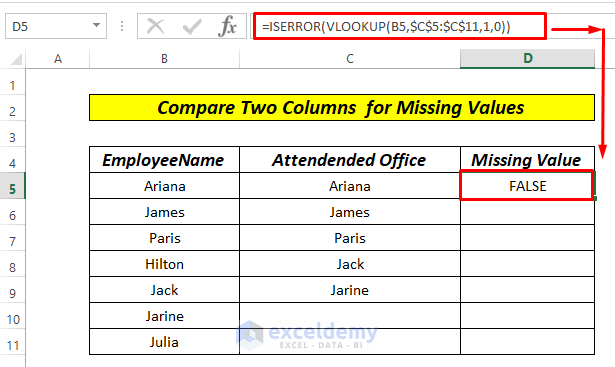
The VLOOKUP function using an absolute cell reference looks up the values in C5:C11. The ISERROR function will return the FALSE if data is present in both columns. Otherwise, TRUE.
- Drag down the Fill Handle to see the result in the rest of the cells.
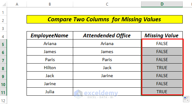 This is the output.
Read More: Excel formula to compare two columns and return a value
Method 2 – Merging the IF, VLOOKUP and ISERROR Functions to Compare Two Columns and Find Missing Values
To see the names that are missing:
- Select D5 and enter the following formula.
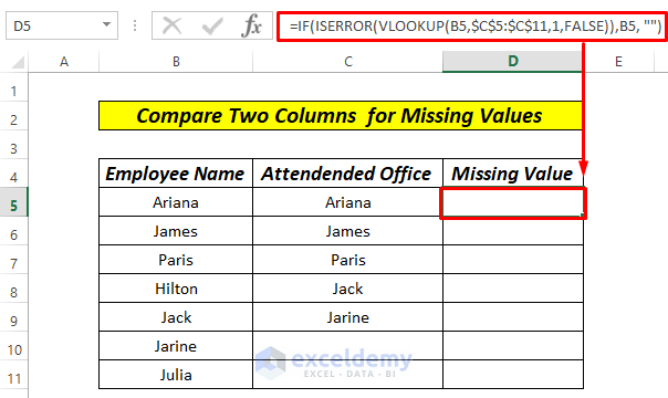
=IF(ISERROR(VLOOKUP(B5,$C$5:$C$11,1,FALSE)),B5, "")
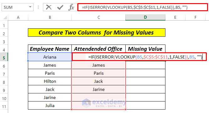
- Press ENTER.
The VLOOKUP function and an absolute cell reference are used like in Method 1 for C5:C11. The ISERROR function returns FALSE if data is present in both columns. Otherwise, TRUE. The IF function returns the name for TRUE and blank for FALSE.
- Drag down the Fill Handle to see the result in the rest of the cells.

Method 3 – Using the MATCH Function to Compare Two Columns in Excel and find Missing Values Steps:
- Select D5 and enter the following formula.
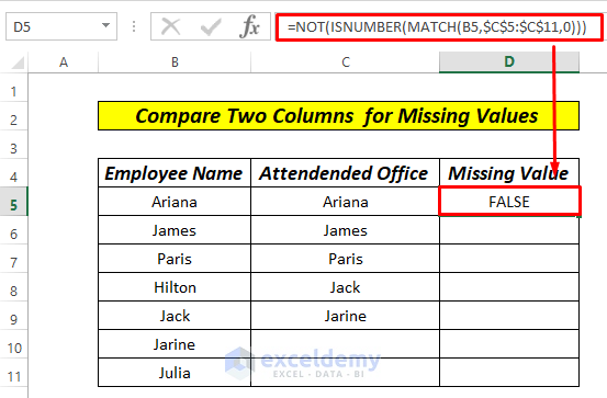
=NOT(ISNUMBER(MATCH(B5,$C$5:$C$11,0)))
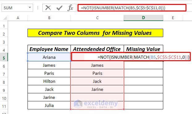
- Press ENTER.
The MATCH function searches for a specified item in a range and returns its relative position in the range. The ISNUMBER returns the matched cell when there is a match, and the NOT function returns TRUE when no match is found.
- Drag down the Fill Handle to see the result in the rest of the cells.
This is the output.
Method 4 – Comparing Two Excel Columns with Conditional Formatting
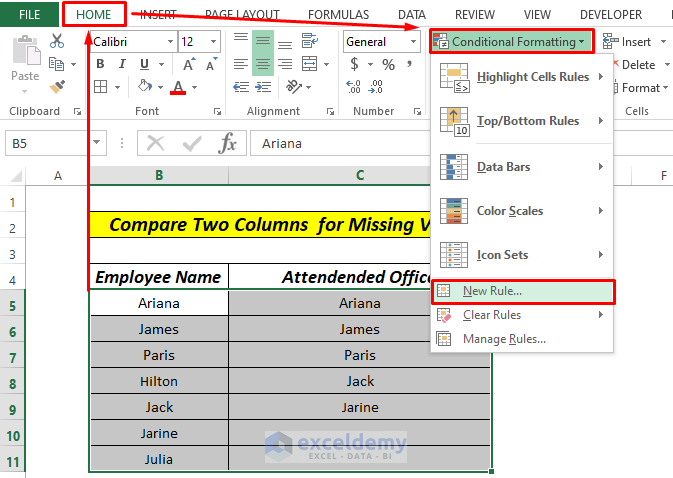
- Select B5:C11.
- Go to Conditional Formatting in the Home tab.
- Select New Rule.
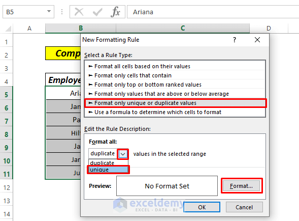
- In the dialog box, select the instructions marked the red in the image below and click Format.
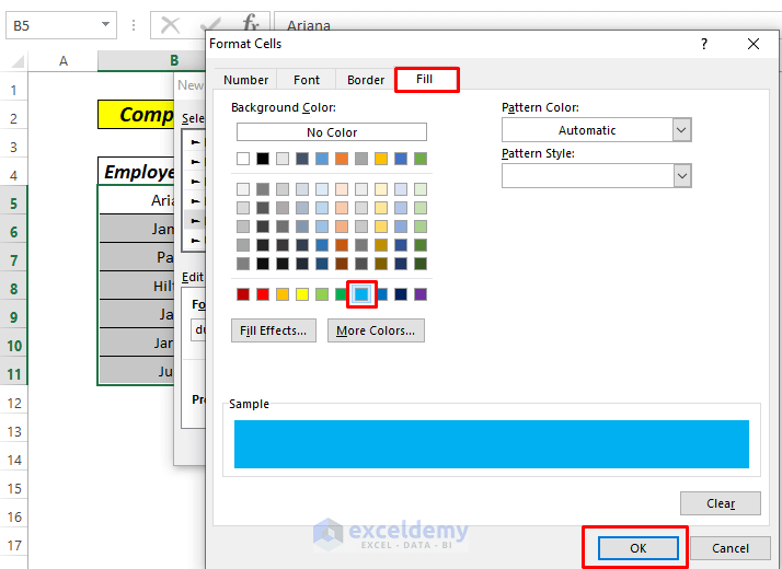
- Select Fill and choose a color.
- Click OK.
This is the output.
Download Practice Workbook
<< Go Back to Columns | Compare | Learn Excel
Get FREE Advanced Excel Exercises with Solutions!

Great, thanks!
Dear Victor,
You are most welcome.
Regards
ExcelDemy