How to Compare 4 Columns in Excel VLOOKUP (7 Methods)

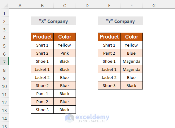
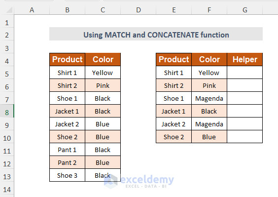
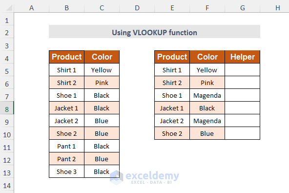
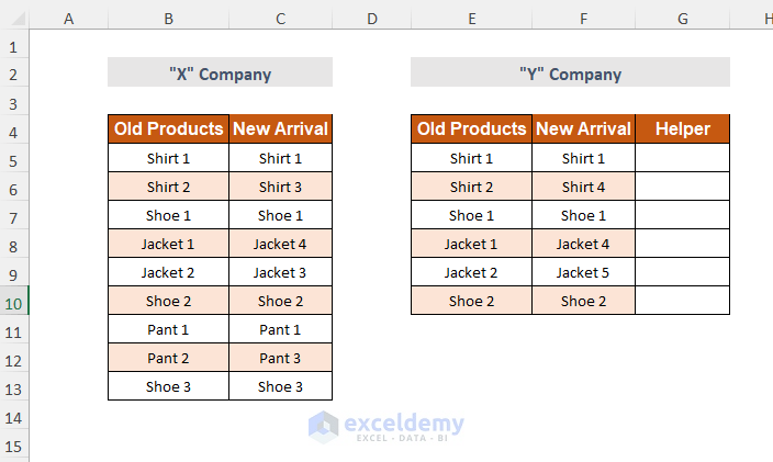
Dataset Overview

In this scenario, we have data from two companies, and we want to compare whether their product names and item colors match. We have a total of 4 columns, and our goal is to identify similarities. Let’s explore the methods for comparing these 4 columns in Excel.

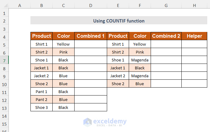
Method 1 – Using the COUNTIF Function

• Add Extra Columns:
  • Create three additional columns: Combined 1, Combined 2, and Helper.

• Combine Text from Product and Color Columns:
  • In the Combined 1 column (starting from cell D5), enter the formula:

This formula concatenates the text from cells B5 and C5, separated by a space.

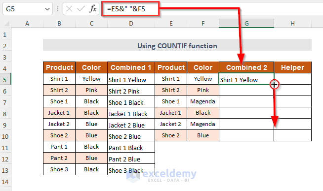
• • Press ENTER and drag down the Fill Handle to apply the formula to all rows.

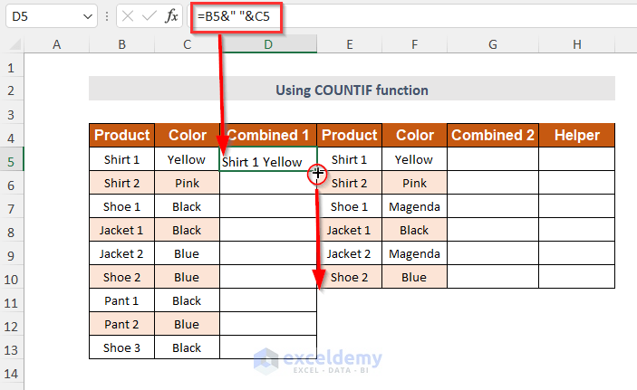
All of the text of the Product and Color column will be combined in the Combined 1 column.

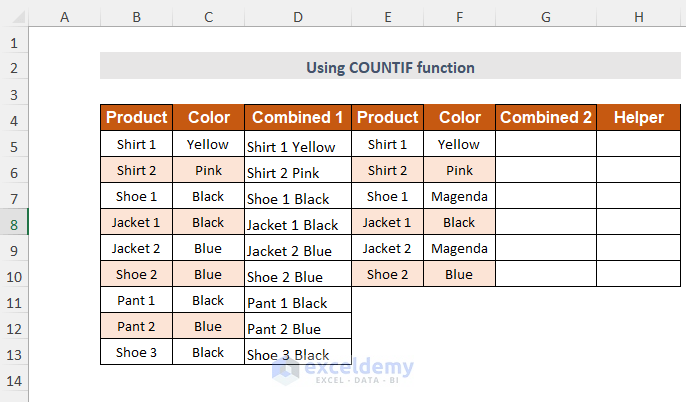
• Combine Text from Other Columns:
  • In the Combined 2 column (starting from cell G5), enter the formula:

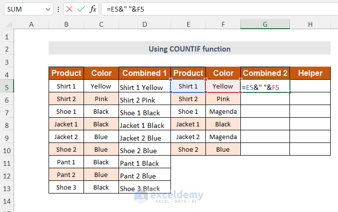
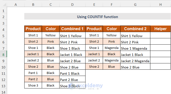
• • Press ENTER and drag down the Fill Handle to apply the formula.

You will get the following results in the Combined 2 column.

• Check for Matches:
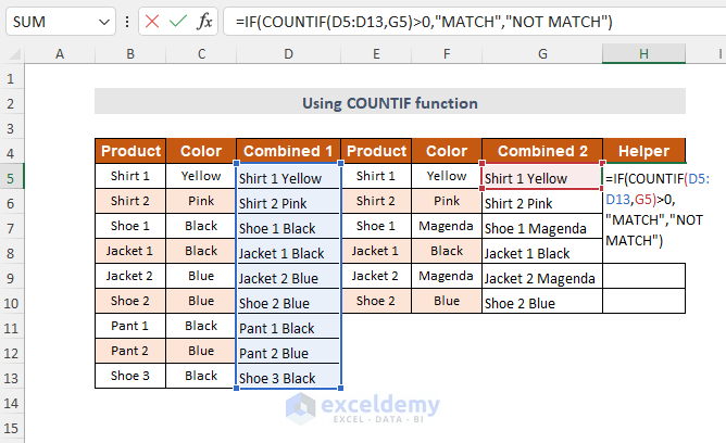
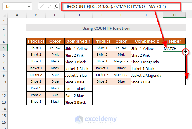
  • In the Helper column (starting from cell H5), insert the formula:

• • Press ENTER and drag down the fill handle to apply the formula to all rows.

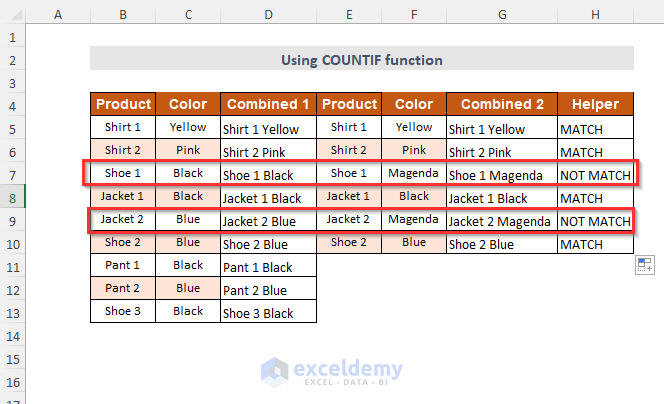
• Result:
  • The Helper column will indicate whether the values match or not.

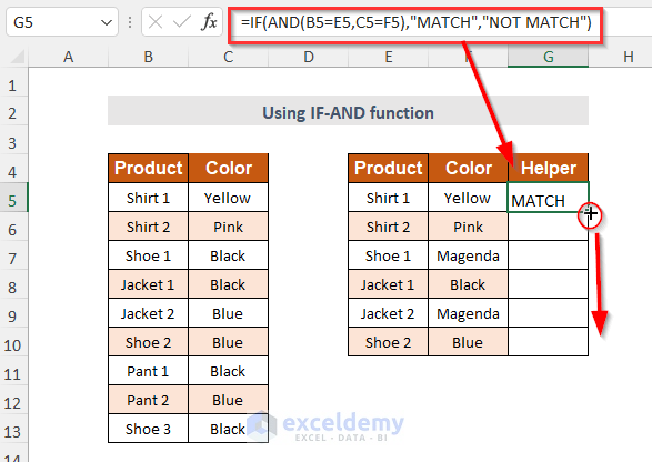
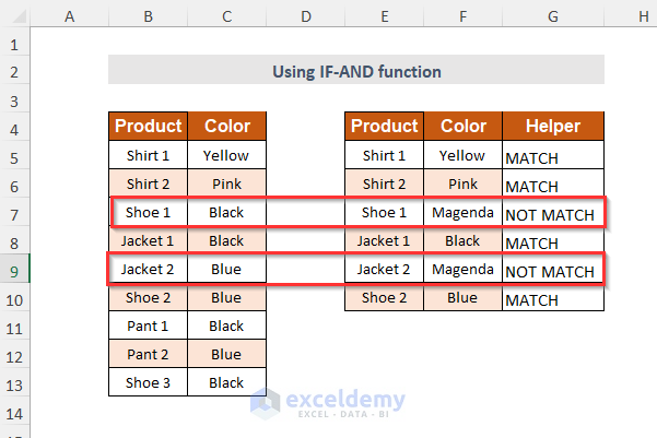
Method 2 – Using the IF-AND Function

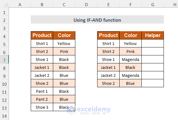
• Add an Extra Column:
  • Create an additional column called Helper.

• Check for Matches:
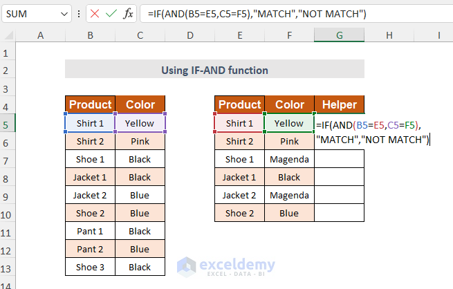
  • In the Helper column (starting from cell G5), enter the formula:

• • Press ENTER and drag down the Fill Handle to apply the formula.

• Result:
  • The Helper column will show whether the values match or not.

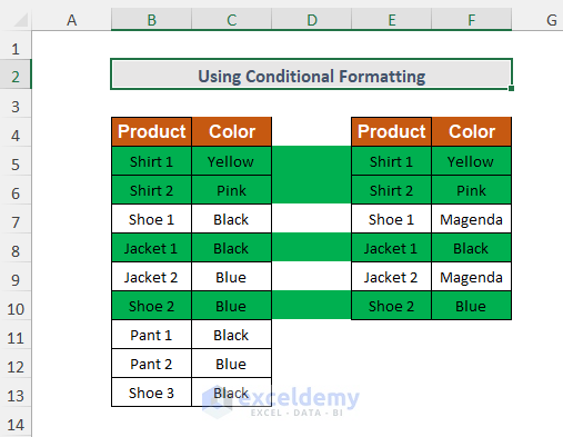
Method 3 – Using Conditional Formatting

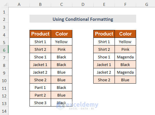
• Select the Columns:
  • Choose the 4 columns (excluding the header) that you want to compare.

• Apply Conditional Formatting:
  • Go to the Home tab.
  • Click on the Conditional Formatting drop-down menu.
  • Choose New Rule.

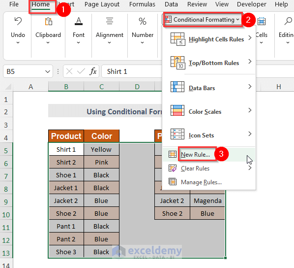
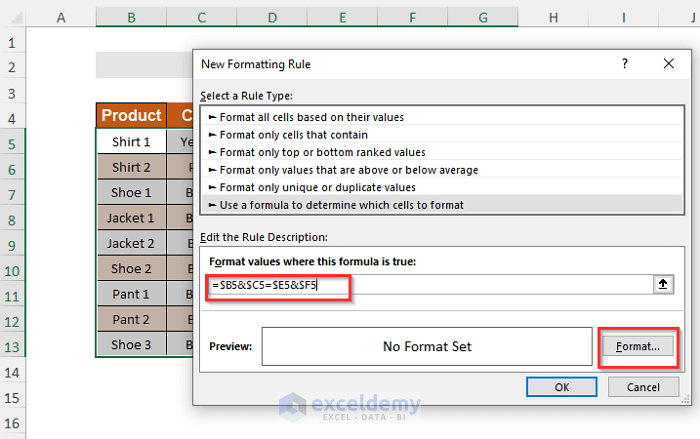
• • In the New Formatting Rule dialog box, select Use a formula to determine which cells to format.

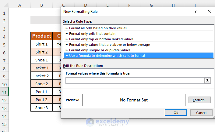
• • Enter the following formula in the Format values where this formula is true:

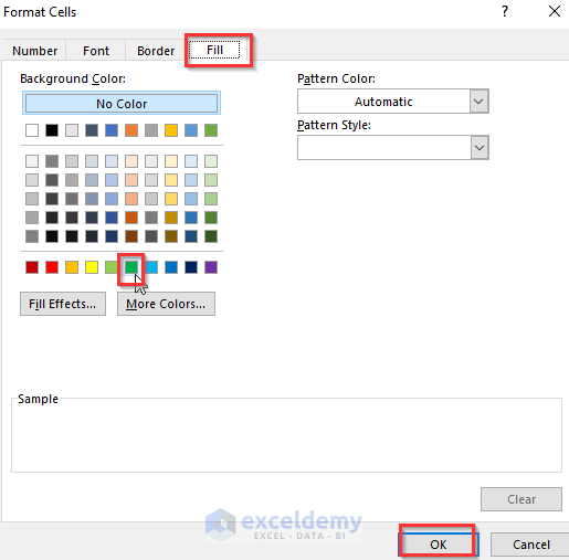
• • Click Format.

• • The Format Cells Wizard will pop up
    • Select the Fill Option.
    • Choose any color as per your choice.
  • Press OK.

• Result:
  • The data table will highlight cells with matching values in these 4 columns using the chosen color.

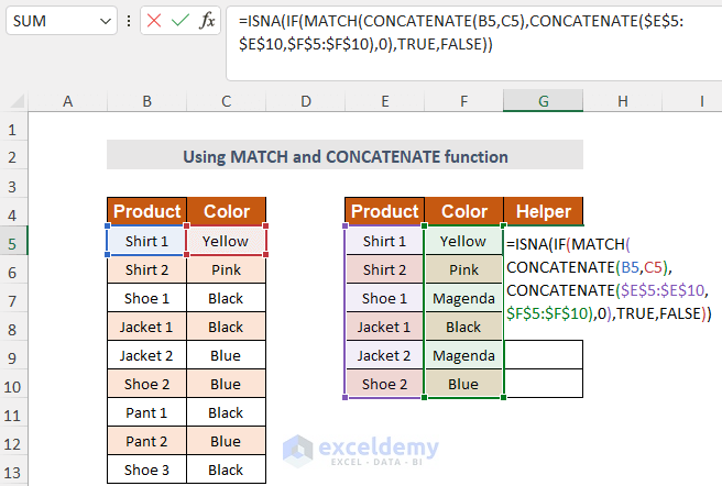
Method 4 – Using the MATCH and CONCATENATE Functions

• Add an Extra Helper Column:
  • Create an additional column called Helper.
• Check for Matches:
  • In the Helper column (starting from cell G5), insert the formula:

• • Press ENTER and drag down the Fill Handle.

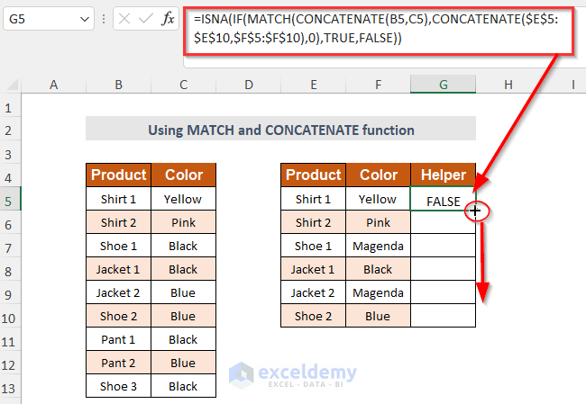
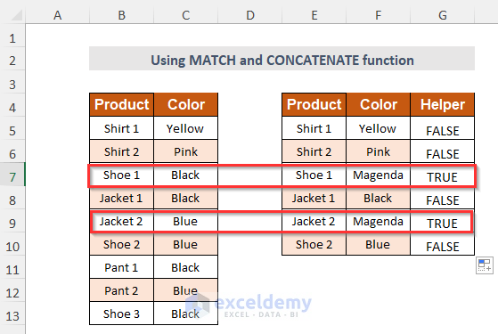
• Result:
  • TRUE indicates non-matching values in these 4 columns.

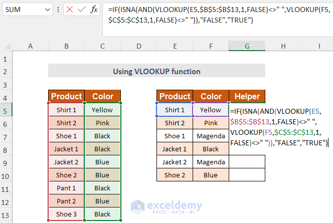
Method 5 – Using the VLOOKUP Function

• Add an Extra Helper Column:
  • Create another column called Helper.
• Check for Matches:
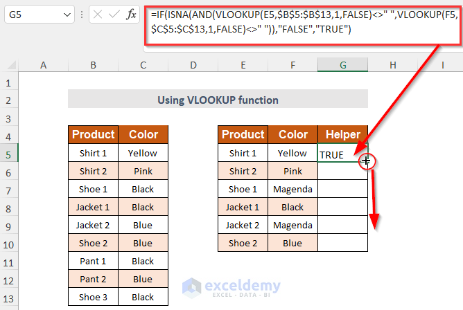
  • In the Helper column (starting from cell G5), enter the formula:

• • Press ENTER and drag down the Fill Handle.

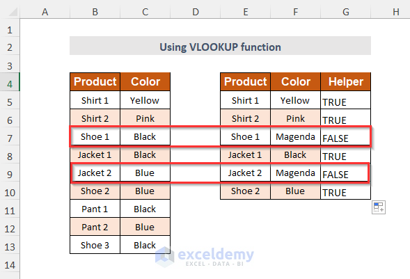
• Result:
  • FALSE indicates non-matching values in these 4 columns.

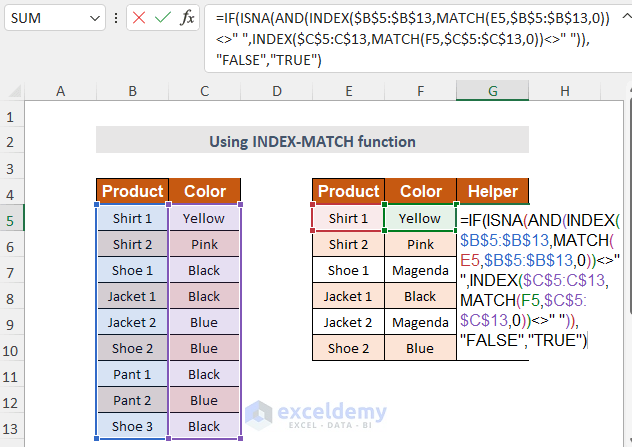
Method 6 – Using the INDEX-MATCH Function

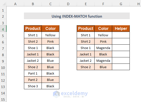
• Add an Extra Helper Column:
  • Create yet another column called Helper.
• Check for Matches:
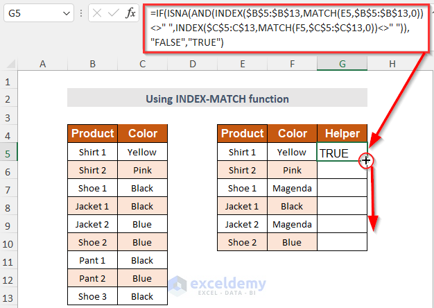
  • In the Helper column (starting from cell G5), insert the formula:

• • Press ENTER and drag down the Fill Handle.

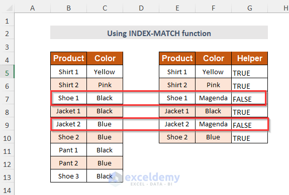
• Result:
  • FALSE indicates non-matching values.

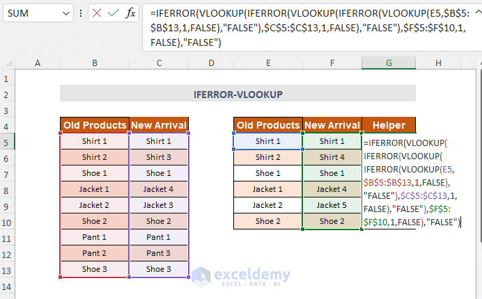
Method 7 – Using the IFERROR-VLOOKUP Function

• Add an Extra Helper Column:
  • Create an additional column called Helper.
• Check for Matches:
  • In the Helper column (starting from cell G5), insert the following formula:

• • Press ENTER and drag down the Fill Handle.

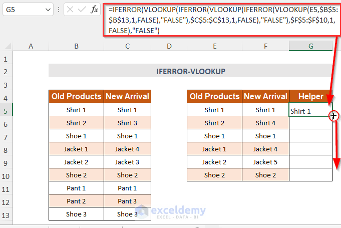
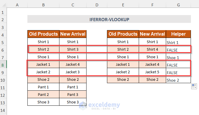
• Result:
  • FALSE indicates non-matching values in these 4 columns.
  • When the columns match, the corresponding text in the cells will appear.

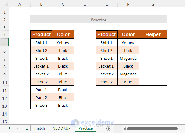
Practice Section

We have provided a Practice section like below in a sheet named “Practice”.

Download Workbook

You can download the practice workbook from here:

<< Go Back to Columns | Compare | Learn Excel