How to Compare Two Columns or Lists in Excel (4 Suitable Ways)

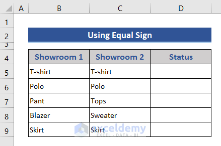
Method 1 – Compare Two Columns Using Equal Operator

Steps:

• Add a new column on the right side to show the matching status.

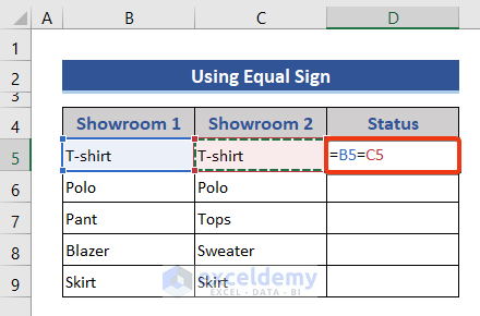
• Enter the following formula in Cell D5.

• Press Enter and drag the Fill Handle icon.

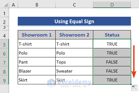
It will output True for match cases otherwise, False.

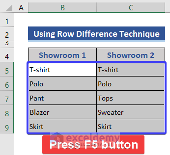
Method 2 – Use Row Differences Command of Go To Special Tool to Compare Two Lists in Excel

Steps:

• Select the whole dataset of Range B5:C9.
• Press the F5 button.

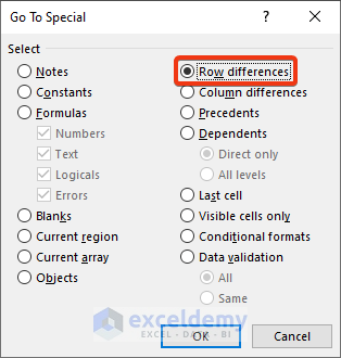
• The Go To dialog box opens. Click on Special.

• Select the Row differences option from the Go To Special window.
• Press OK.

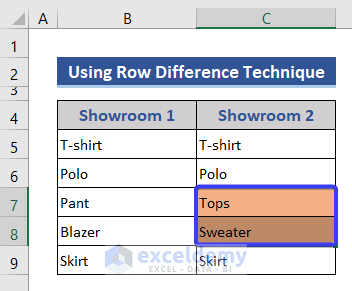
You can see two cells of the second column are selected.

• Change the color of the cells from the Fill Color option.

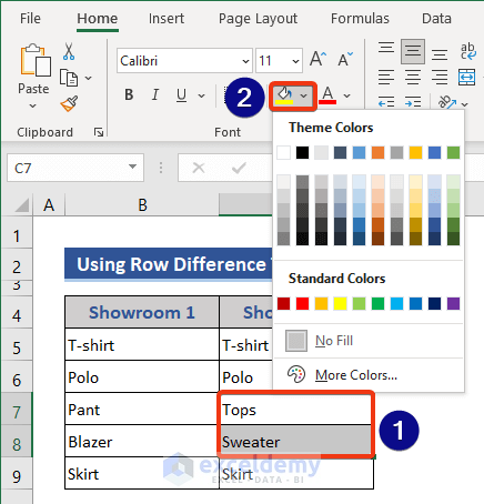
• Cells of the second column with mismatched data will be highlighted.

Method 3 – Use Excel Functions to Compare Two Columns or Lists in Excel

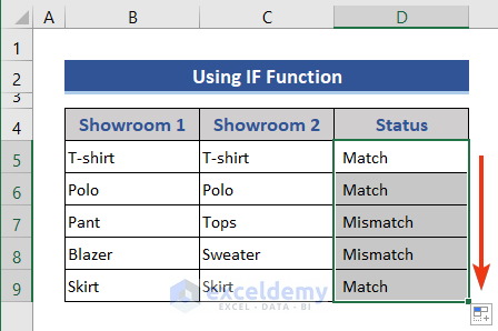
3.1 Using IF Function

The IF function will compare the cells of the columns row-wise and check whether they are the same or not.

Steps:

• Enter the formula below in Cell D5.

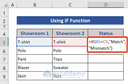
This formula will check whether the cells are the same or not. If same, it shows Match otherwise, Mismatch.

• Drag the Fill Handle icon downwards.

The following formula is to compare for not matching values.

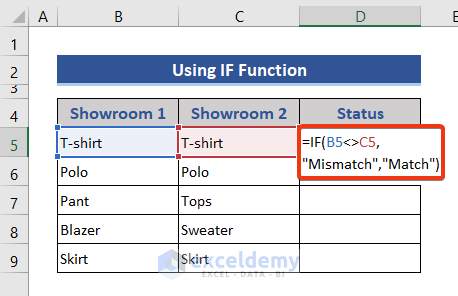
In this case, when the condition is True, it shows Mismatch, otherwise Match.

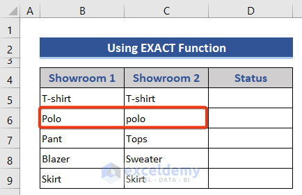
3.2 Applying EXACT Function

When you have the same data in two columns with case differences, use the EXACT function .

In Row 6, we have the same data from different cases. Enter the EXACT function to check the result.

Steps:

• Insert the formula below in Cell D5.

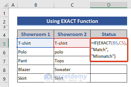
The IF function is used to show the comment based on the decision taken by the EXACT function.

• Drag the Fill Handle

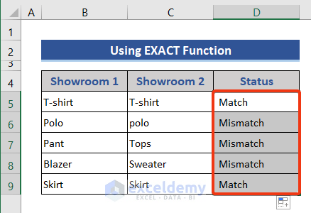
We get the result as Mismatch.

3.3 Using MATCH Function

We will compare the 1st column with the 2nd column. When a match of the 1st column is found in the 2nd column, the result will be TRUE.

We will use the MATCH function with ISERROR and IF functions.

Steps:

• Enter the following formula in Cell D5.

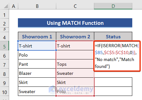
When the statement is true result will be Match found otherwise No match.

• Press Enter to execute the formula.

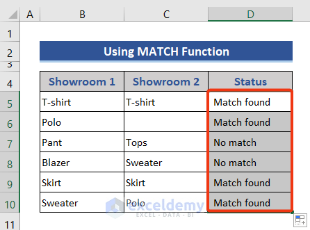
We got the result based on the 1st column. We are looking for a match in the 2nd column.

Read More: Excel formula to compare two columns and return a value

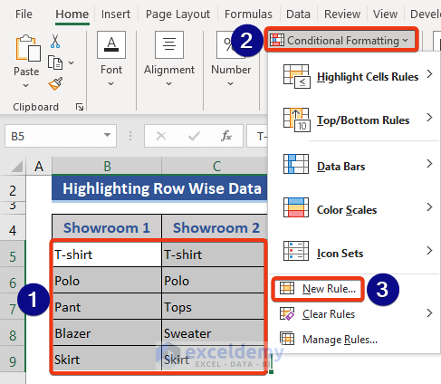
Method 4 – Compare Two Columns and Highlight Using Conditional Formatting

4.1 Highlight Equal Values in Two Columns

Steps:

• Select the dataset.
• Go to the Conditional Formatting option from the Home tab.
• Choose New Rule from the dropdown.

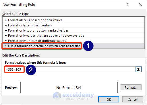
• The New Formatting Rule window will open.
• Select Use a formula to determine which cells to format as the rule type.
• Enter the following formula on the marked box.

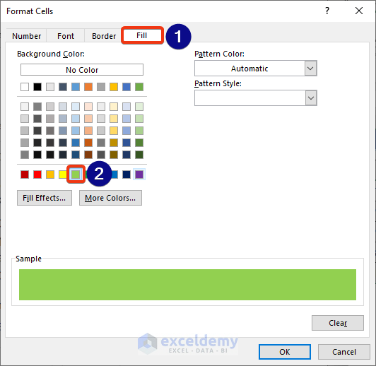
• Choose the Fill tab from the Format Cells window.
• Choose the color.
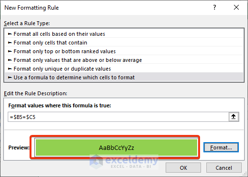
• Press OK.

• Press OK.

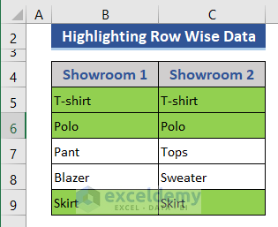
Cells with the same data will be highlighted.

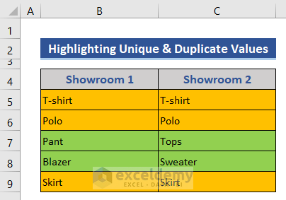
4.2 Highlight Unique and Duplicate Cells

Steps:

• Enter the New Rule option.

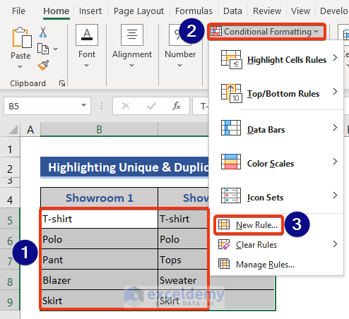
• Select Format only unique or duplicate values rule type.
• Choose the duplicate option.

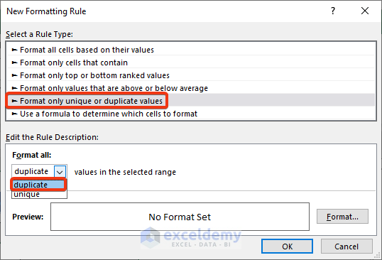
• Set the format color and press OK.

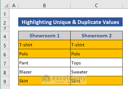
Duplicate cells are highlighted.

• Follow the previous process and choose the unique option.

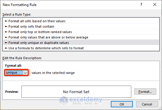
Duplicate and unique data care are highlighted in different colors.

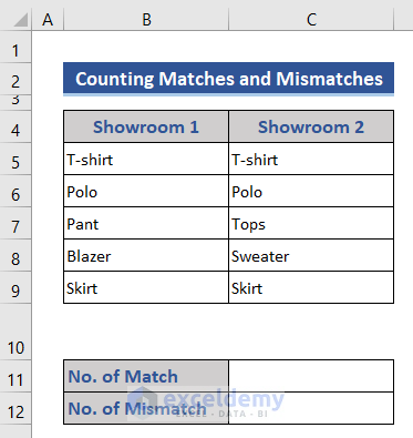
Compare Two Columns in Excel and Count Matches

In this function, we will use the combination of the SUMPRODUCT function, and the COUNTIF function to count the matches. After that, we will calculate the number of total rows using the ROWS function and subtract the matches to get the number of mismatches.

Steps:

• Add two rows. One for the match and another for the mismatch.

• Insert the following formula based on the SUMPRODUCT and COUNTIF function in Cell C11.

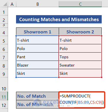
• Press Enter to get the result.

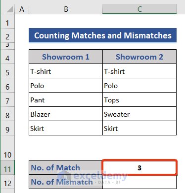
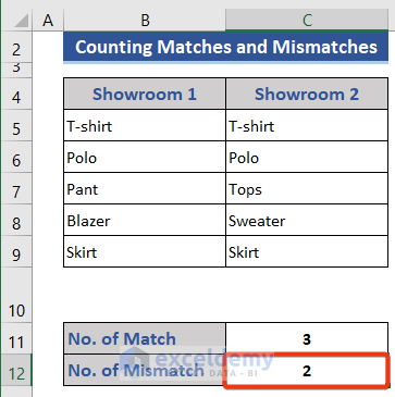
We get the number of matched rows.

• Go to Cell C12 and enter the formula below.

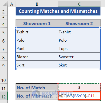
• PressEnter to get the number of mismatches.

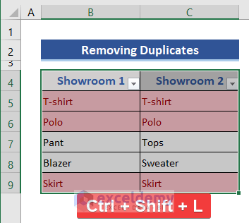
Compare Two Columns in Excel and Remove Duplicates

Steps:

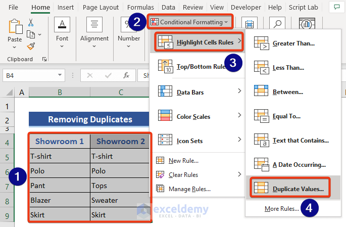
• Select the dataset.
• Go to the Conditional Formatting section.
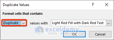
• Choose Duplicate Values from the Highlight Cells Rules.

• Choose a color to indicate the duplicates.

• The color of cells containing duplicate data has been changed.
• Press Ctrl + Shift+ L to enable the filter option.

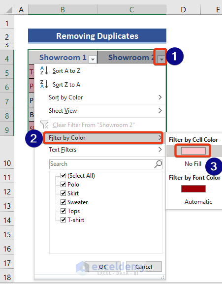
• Click on the down arrow of the 2nd column.
• Choose the color of the duplicate cells from the Filter by color section.

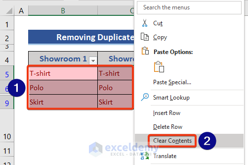
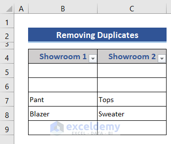
• Only duplicate values are shown. Select that range.
• Right-click on the mouse.
• Choose the Clear Contents option from the Context Menu.

• Duplicate values are removed from the dataset.

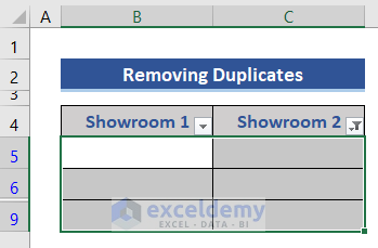
• Go to the filter section and check the Select All option.

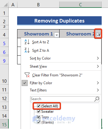
• No duplicates are showing now.

Excel Match Two Columns and Extract Output from a Third with VLOOKUP

Steps:

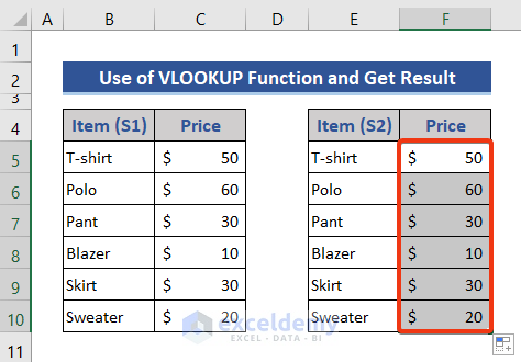
• Enter the following formula based on the VLOOKUP function on Cell F5.

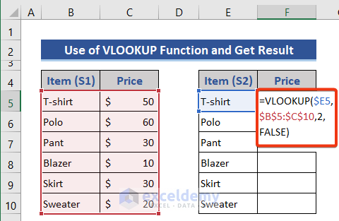
• It compares Item (S1) with Item (S2) and extracts the price in the 2nd table.

How to Compare More Than Two Columns in Excel

Method 1 – Use Excel AND Function

After checking all the conditions, the result will be shown based on the comment used in the IF function. Before applying the formula, we add another column named Showroom 3.

Steps:

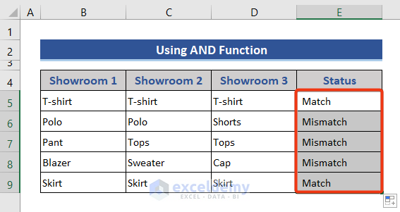
• Enter the following formula on Cell E5.

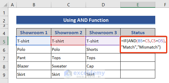
• Drag the Fill Handle icon.

Method 2 – Compare with Excel COUNTIF Function

The COUNTIF function counts the number of cells within a range that meet the given condition, and  the COUNTA function counts the number of cells in a range that are not empty.[/wpsm_box]

We will use these functions to compare multiple columns.

Steps:

• Enter the following formula on Cell E5.

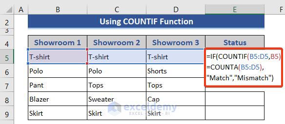
• Drag the Fill Handle icon.

Download Practice Workbook

<< Go Back to Columns | Compare | Learn Excel