Latest Posts From Md. Nafis Soumik
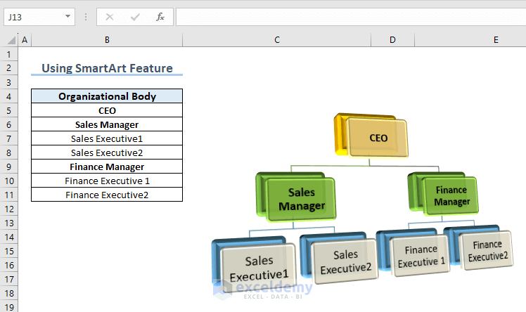
What Is Hierarchy? Hierarchical Chart: The term hierarchy has a dual meaning. First, it refers to a specific type of chart used to ...

By following this article, you will learn to calculate weighted average in Excel. We’ll use a simple formula, SUM function, and the combination of SUMPRODUCT ...

Error bars represent uncertainty and variability in data. They provide a visual indication of measurement uncertainty, statistical significance, comparative ...

This is an overview. Click the image for a detailed view Download Practice Workbook Excel Interpolation.xlsx What Is Interpolation? ...

This is an overview. There is a list of 10 patients and their height in cm. A frequency distribution table was created by grouping the height into 4 ...

Here's an overview of copying a sheet. Download the Practice Book Copy Sheet.xlsx How to Copy a Sheet in the Same Workbook in Excel ...
This is an overview. Method 1 - Combining the LEFT, MID, FIND & LEN Functions to Abbreviate in Excel Enter the following ...

In the following overview image, we have compared two different lists containing the available products in a store and ordered products. If the ordered ...

In this Excel tutorial, you will learn - About the default options in the status bar that appear whenever you open the Excel application - How to customize ...

Download Practice Book Conditional Formatting with Named Range.xlsx Example 1 - Using Array Formula with Named Range in Conditional Formatting ...

In this article, we will explore how to use the PERMUTATIONA function in Excel to generate phone numbers, pin codes, license plate numbers, and even Powerball ...

Want to learn the use Case vs If statement in Excel VBA? Then, this is the right place for you. One of the fundamental concepts in VBA is making decisions ...

Excel VBA provides various methods to wrap text in cells, ranges, and entire worksheets. Knowing these methods can help you customize the appearance of your ...

In this article, we'll demonstrate how to create an availability schedule template in Excel, as in the video and image below. Watch Video – Make an ...

Are you tired of performing repetitive tasks every time you open an Excel workbook? Do you want to automate your workflow and save time? If your answer is yes, ...
See Our Reviews at


Hi Kevin!
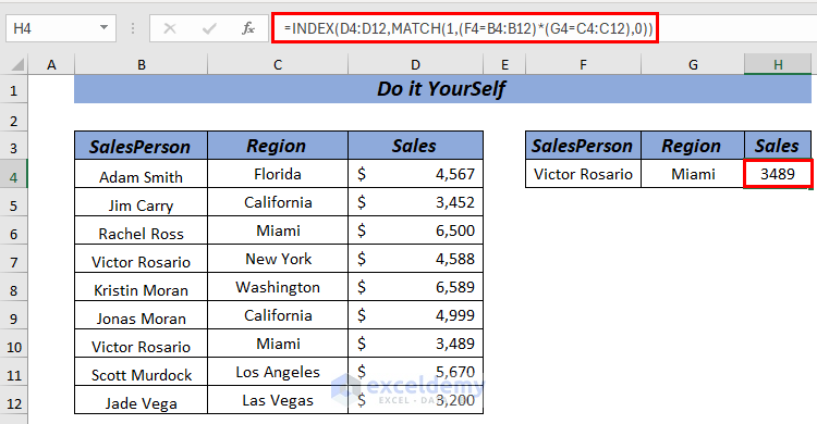
It brings me great joy to know that you found our blog helpful. You are most welcome. As for your query, you can use the following formula:
=INDEX(D4:D12,MATCH(1,(F4=B4:B12)*(G4=C4:C12),0))To be more clear about the cell references look at the image below:
Regards,
Nafis
ExcelDemy
Hi MAHMUD,
Thank you for your valuable suggestion. I updated the formula for calculating electricity bill with Variable Unit Price (Slab). Hope you find this article useful.
Regards,
ExcelDemy
Hi Liam,
Thank you for taking the time to comment on our blog and for suggesting a shorter method for the task that is demonstrated. We appreciate your input and always welcome new ideas.
After carefully considering your formula, I noticed there was a backslash “\” missing from the col_delimiter argument of the TEXTSPLIT() function inside the formula. To ensure the best results, modify your formula like this:
=CHOOSECOLS(TEXTSPLIT(A1,"\"),-1)(Assuming the full path address is inside the cell A1).We value your engagement and encourage you to keep sharing your thoughts and ideas. It’s through constructive discussions like this that we can all learn and improve. Thanks again for your comment!
Regards,
ExcelDemy.
Hi Mahmoud,
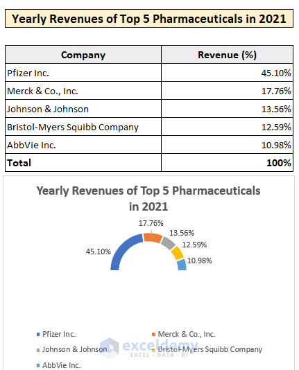
You can create a half doughnut chart to show the correct percentages with data labels by following the steps mentioned in this article. Only exception is you will need a different data table with the yearly revenues converted into percentages of the total.
You can do this by applying the following formula inside any cell:
=C5/$C$10. Use fill handle to populate the dataset and keep the percentage column into percentage format. Now follow the exact steps described in this article. Upon finishing check the Data Labels option from Chart Element. Your half doughnut chart with percentage Data labels is now ready.I hope it solves your problem.
Regards,
ExcelDemy.
Hello JK,
Which formula are you talking about?
Do you have a formula for yourself that you want to convert?
Or, Do you want to convert any of the formulas from the post?
Please let us know. We would be happy to help.
Regards
Exceldemy
Hi Jenn,
Based on your comment, it seems you are looking for a way to create a spreadsheet that displays different tables based on the selected company.
To address your requirement, one approach is to use Excel’s “Data Validation” feature combined with “Index” and “Offset” functions. Here’s a potential step-by-step solution:
1. Set up your spreadsheet with separate tables for each company, each in a different range of cells.
2. Create a list of company names (e.g., in a dropdown) where the user can select the desired company.
3. Assign data validation to the cell where the user selects the company, limiting the input to the list of company names.
4. Next, use the “Index” and “Offset” functions to display the corresponding table based on the selected company.
Here’s an example of how this could work:
1. Create separate tables for each company, each in a different range of cells (e.g., Company A in cells A1:D10, Company B in cells A15:D24, Company C in cells A29:D38).
2. Create a dropdown list of company names (e.g., in cell A50) using Excel’s Data Validation feature.
3. Use the “Index” and “Offset” functions to retrieve the appropriate table based on the selected company. For example, in cell A55, you could use the following formula:
=INDEX($A$1:$D$10, OFFSET($A$1:$A$10, MATCH($A$50,$A$1:$A$10,0)-1, 0, ROWS($A$1:$A$10), COLUMNS($A$1:$D$10)))This formula will retrieve the table for the selected company dynamically.
Now, when you select a company from the dropdown list in cell A50, the corresponding table will be displayed in cell A55 and automatically update based on the selection.
Please note that the specific ranges and formulas may need to be adjusted based on the actual structure and layout of the spreadsheet. However, this approach should provide a starting point to achieve the desired functionality of displaying different tables based on the selected company in Excel.
Regards,
ExcelDemy
Hello Kumar,
Both the formulas you mentioned work fine and generate same results. Try again. If it still does not work, please send us your Excel file at [email protected]
And yes. There is a simpler formula to find out the original price directly without calculating the GST amount. Use this formula inside cell C7: Original price = C4/(1+C5)
Thank you.
Regards,
Exceldemy
Hello Ed McCann,
It’s possible that the Pivot table is referencing a range of cells that includes data outside of the intended range. Here are a few steps you can try to troubleshoot the issue:
1. Check the source data range: Make sure that the Pivot table is referencing the correct range of cells that contain your data. Select any cell inside the Pivot table, go to the “Analyze” or “Options” tab in the ribbon, and look for the “Change Data Source” or “Select Data” button. Clicking on this button will show you the range of cells that the Pivot table is using as its data source.
2. Check for hidden data: It’s possible that there is hidden data in the source data range that is being included in the Pivot table. Select the source data range, go to the “Home” tab in the ribbon, and click on the “Format” dropdown. From here, click on “Hide & Unhide” and then “Unhide Rows/Columns” to reveal any hidden data.
3. Refresh the Pivot table: If none of the above steps work, try refreshing the Pivot table. Select any cell inside the Pivot table, go to the “Analyze” or “Options” tab in the ribbon, and click on the “Refresh” button. This will recalculate the Pivot table based on the current data source.
I hope these steps help you troubleshoot the issue with your Pivot table.
If the problem persists, then you can send your excel workbook to this email: [email protected]
Regards
Exceldemy