How to Apply Abbreviation in Excel - Abbreviate Words and Numbers

This is an overview.

excel abbreviation

⏷Apply Abbreviation for Initial Word
⏵Combine LEFT, MID, FIND & LEN Functions
⏵Combine CONCATENATE, LEFT, MID, FIND & LEN Functions
⏷Apply Abbreviations for All Words
⏵Combine Multiple Functions to Abbreviate All Words (Microsoft 365 and Excel 2019)
⏵Combine Multiple Functions to Abbreviate All Words (All Excel Versions)
⏵Apply Custom VBA Function to Abbreviate All Words
⏷Abbreviate Days in Excel
⏵Use TEXT Function
⏵Combine CHOOSE & WEEKDAY Functions
⏷Apply Abbreviation for Numbers
⏵Abbreviate Numbers in Thousands
⏵Abbreviate Numbers in Millions
⏵Abbreviate Numbers in Billions
⏵Abbreviate Numbers in Billions, Millions, or Thousands According to Value
⏷Find Corresponding Abbreviation from a List
⏵Use VLOOKUP Function
⏵Use XLOOKUP Function
⏵Combine INDEX & MATCH Functions
⏷Things to Remember
⏷Frequently Asked Questions
⏷Excel Abbreviation: Knowledge Hub

How to Apply an Abbreviation to an Initial Word in Excel

Initialism format of abbreviation is a special type of abbreviation in which only the first word is abbreviated. For example: Walmart Inc. >> W. Inc. Two methods can be used to apply this format.

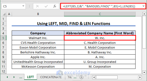
Method 1 – Combining the LEFT, MID, FIND & LEN Functions to Abbreviate in Excel

Enter the following formula in C5:

=LEFT(B5,1)&". "&MID(B5,FIND(" ",B5)+1,LEN(B5))

Press Enter and use the Fill Handle.

Formula Breakdown

LEFT(B5,1): The LEFT function extracts the first character (initial) from the text in B5.
“. “: a period (dot) and a space are placed after the initial.
MID(B5, FIND(” “,B5)+1, LEN(B5)): This section extracts the portion of the name after the space.
FIND(” “,B5)+1: The FIND function locates the position of the first space in the text and adds 1 to this position to determine the starting point of the name (after the space).
LEN(B5): The LEN function calculates the total length of the text in B5.
MID (…): The MID function extracts a portion of the text starting from the position calculated above, and its length extends until the end of the text.

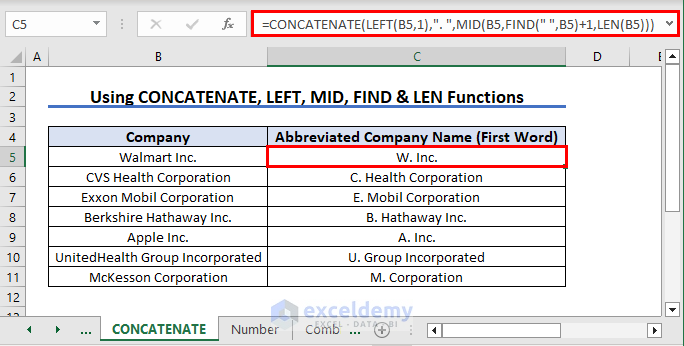
Method 2 – Combining the CONCATENATE, LEFT, MID, FIND & LEN Functions

Enter the following formula in C5:

=CONCATENATE(LEFT(B5,1),". ",MID(B5,FIND(" ",B5)+1,LEN(B5)))

Press Enter and use the Fill Handle.

Formula Breakdown

LEFT(B5,1): extracts the first character (initial) from the text in B5.
“. “: adds a period and a space to separate the initial from the rest of the name.
MID(B5, FIND(” “,B5)+1, LEN(B5)): extracts the portion of the name after the space.
FIND(” “,B5)+1: The FIND function locates the position of the first space in the text and adds 1 to this position to determine the starting letter of the name (after the space).
LEN(B5): The LEN function calculates the total length of the text in B5.
MID(…): The MID function extracts a portion of the text starting from the position calculated above, and its length extends until the end of the text.
CONCATENATE(…): The CONCATENATE function combines the results of the previous steps into a single string.

How to Apply Abbreviations to All Words in Excel

There are 3 methods to apply abbreviations to all words in a word group.

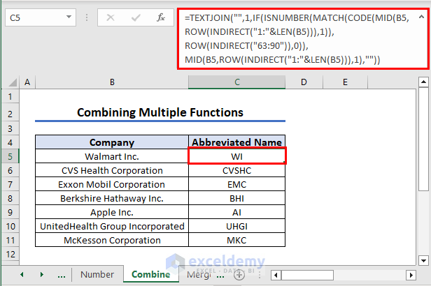
Method 1 – Combining the TEXTJOIN, ISNUMBER, MATCH, CODE, MID, ROW, INDIRECT, LEN, and ROW Functions

Use the following formula in C5:

=TEXTJOIN("",1,IF(ISNUMBER(MATCH(CODE(MID(B5,ROW(INDIRECT("1:"&LEN(B5))),1)),ROW(INDIRECT("63:90")),0)),MID(B5,ROW(INDIRECT("1:"&LEN(B5))),1),""))

Press Enter and use the Fill Handle.

Formula Breakdown

LEN(B5) – The LEN function calculates text length in B5.
ROW(INDIRECT(“1:”&LEN(B5))) – generates an array of sequential numbers from 1 to the length of the text in B5. It is created using the ROW function and the INDIRECT function, which converts the range string “1:” concatenated with the length of B5 into an actual range.
MID(B5,ROW(INDIRECT(“1:”&LEN(B5))),1) – The MID function extracts individual characters from B5. It takes three arguments: the text to extract from (B5), the starting position (generated by ROW(INDIRECT(“1:”&LEN(B5)))), and the number of characters to extract (1).
CODE(MID(…)) – The CODE function converts each extracted character into its corresponding Unicode value and applies it to the result obtained from the MID function.
ROW(INDIRECT(“63:90”)) – generates an array of numbers from 63 to 90, which represent the Unicode values for uppercase letters in the ASCII character set.
MATCH(CODE(…),ROW(INDIRECT(“63:90”)),0) – The MATCH function checks if each Unicode value obtained in step 4 is present within the array of uppercase letter Unicode values in step 5. It returns the position of the match or an error if there is no match. The value of 0 as the third argument ensures an exact match.
ISNUMBER(MATCH(…)) – The ISNUMBER function checks if the result of the MATCH function in step 6 is a number. If there is a match, it returns TRUE; otherwise, it returns FALSE.
IF(ISNUMBER(…),MID(…),””) – The IF function evaluates the result from step 7. If it is TRUE (meaning there was a match), the MID function is used again to extract the character from B5. Otherwise, an empty string (” “) is returned.
TEXTJOIN(“”,1,IF(…)) – The TEXTJOIN function combines all the non-empty characters obtained in step 8 into a single text string. The separator argument is an empty string (” “), and the ignore_empty argument is set to 1 to exclude empty values.

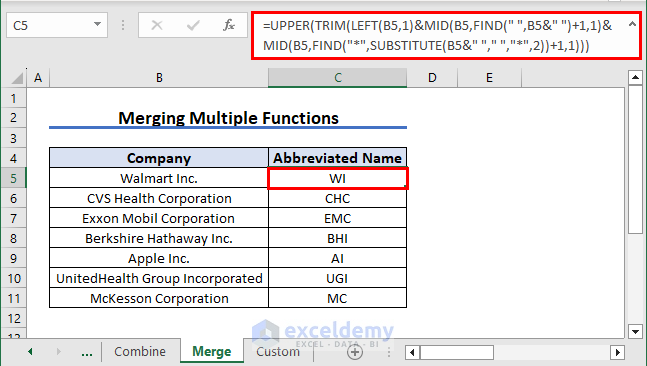
Method 2 – Combining the UPPER, TRIM, LEFT, MID, FIND, and SUBSTITUTE Functions

Enter the following formula in C5:

=UPPER(TRIM(LEFT(B5,1)&MID(B5,FIND(" ",B5&" ")+1,1)&MID(B5, FIND("*", SUBSTITUTE(B5&" "," ","*",2))+1,1)))

Press Enter and use the Fill Handle.

Formula Breakdown

LEFT(B5,1) – The LEFT function extracts the first character from B5. It takes two arguments: the text to extract from (B5) and the number of characters to extract (1). It captures the first letter of the text.
MID(B5,FIND(” “,B5&” “)+1,1) – The MID function extracts a single character within a text string. It takes three arguments: the text to extract from (B5), the starting position (obtained by finding the first space using FIND), and the number of characters to extract (1). It returns the character after the first space.
MID(B5, FIND(“*”, SUBSTITUTE(B5&” “,” “,”*”,2))+1,1) – extracts a single character from within a text string. The starting position is obtained by finding the second occurrence of a space (replaced by an asterisk using the SUBSTITUTE function) and adding 1. It returns the character after the second space.
TRIM(…) – The TRIM function removes any extra spaces before and after the extracted characters and ensures the resulting abbreviation does not have leading or trailing spaces.
UPPER(…) – The UPPER function converts the abbreviation to uppercase.

You can apply this method in all Excel versions.

Method 3 – Applying a Custom Function Using VBA

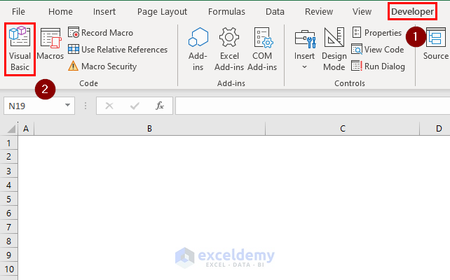
Go to the Developer tab >> select Visual Basic.

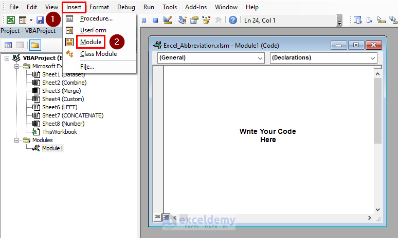
Select Insert >> Module.

If you are using VBA for the first time, add the Developer tab to the ribbon.

Enter the following code in Module1:

Code Syntax:

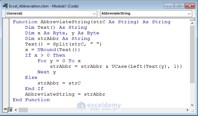
Function AbbreviateString(strC As String) As String
Dim Text() As String
Dim x As Byte, y As Byte
Dim strAbbr As String
Text() = Split(strC, " ")
x = UBound(Text())
If x > 0 Then
For y = 0 To x
strAbbr = strAbbr & UCase(Left(Text(y), 1))
Next y
Else
strAbbr = strC
End If
AbbreviateString = strAbbr
End Function

Code Breakdown

This VBA code defines a function called AbbreviateString that takes a string (strC) as input and returns an abbreviated version of the string.
The function declares variables, including an array Text() to store the individual words of the string and x and y as counters.
The Split function is used to split the input string into an array of words, using space (” “) as delimiter. The result is stored in the Text() array.
The variable x is assigned the upper bound of the Text() array, which represents the number of words in the string.
If there is more than one word (x > 0), the code performs a loop from 0 to x and appends the uppercase first letter of each word to the strAbbr string variable.
If there is only one word in the string (x = 0), the strAbbr variable is assigned the value of the input string.
The function returns the strAbbr string, which contains the abbreviated version of the input string.

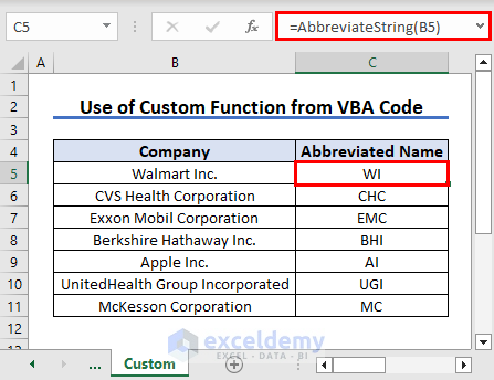
Go back to the Custom sheet. Use the following formula in C5:

=AbbreviateString(B5)

Press Enter and use the Fill Handle.

This is the output.

AbbreviateString() is the User Defined Function that we have created using VBA beforehand.

How to Abbreviate Days in Excel

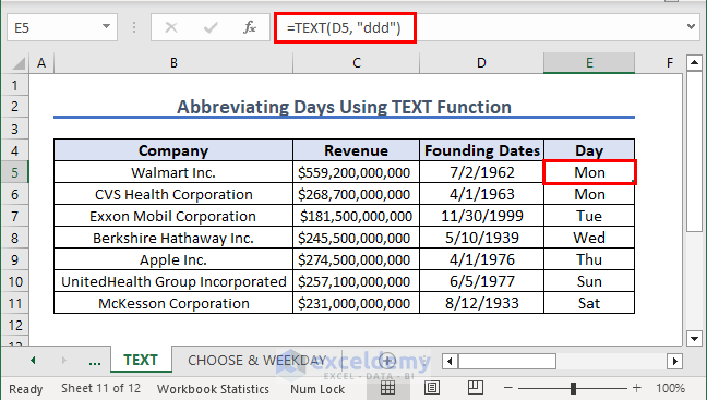
Method 1 – Using the TEXT Function

In E5, enter the following formula:

=TEXT(D5, “ddd”)

Press ENTER >> use the Fill Handle.

The names of the days are abbreviated.

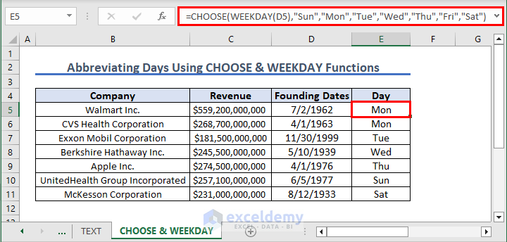
Method 2 – Combining the CHOOSE & WEEKDAY Functions

In E5, use the following formula:

=CHOOSE(WEEKDAY(D5),"Sun","Mon","Tue","Wed","Thu","Fri","Sat")

Press ENTER. Use the Fill Handle.

The names of the days are abbreviated.

Formula Breakdown

WEEKDAY(D5): Calculates the weekday of the date in D5. The WEEKDAY function returns a number representing the day of the week: Sunday is 1, Monday is 2, Tuesday is 3, and so on.
CHOOSE(…): The CHOOSE function selects a value from a list based on a specified index number. Here, the index number is the result of the WEEKDAY function (the day of the week).
“Sun”, “Mon”, “Tue”, “Wed”, “Thu”, “Fri”, “Sat”: These are the values to select from.

How to Apply Abbreviation to Numbers in Excel

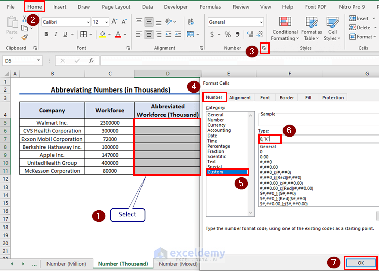
Method 1 – Abbreviating Numbers in Thousands (K)

Select D5:D11 >> click Home >> Small Arrow (Number group).
In Format Cells, select Number >> Custom.
Enter the formula in Type:

0,"K"

Click OK.

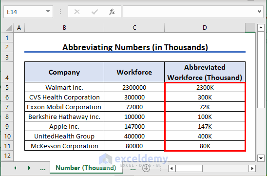
Copy C5:C11 and paste it in D5:D11.

All numbers are abbreviated.

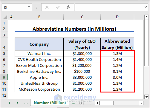
Method 2 – Abbreviating Numbers in Millions (M)

Select D5:D11 >> click Home >> Small Arrow (Number group).
In Format Cells, select Number >> Custom, and enter the following in Type:

0.0,,"M"

Click OK.

Copy C5:C11 and paste it in D5:D11.

All numbers are abbreviated.

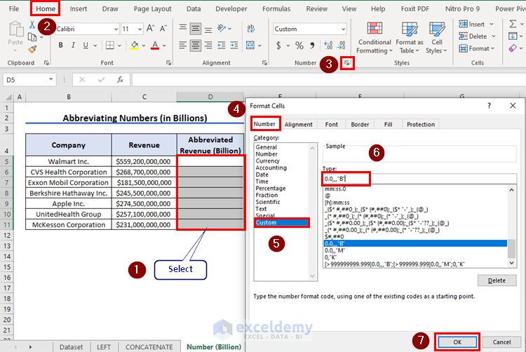
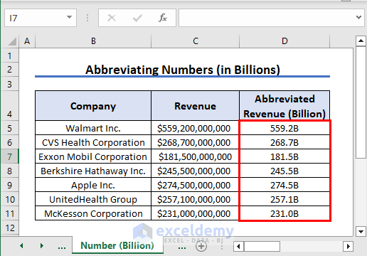
Method 3 – Abbreviating Numbers in Billions (B)

Select D5:D11 >> click Home >> Small Arrow (Number group).
In Format Cells, select Number >> Custom, and enter the following in Type:

0.0,,,"B"

Click OK.

Copy C5:C11 and paste it in D5:D11.

All numbers are abbreviated.

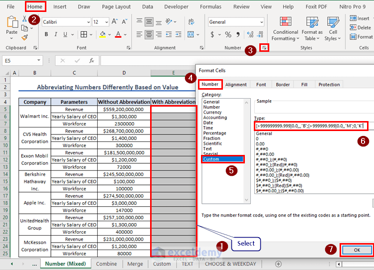
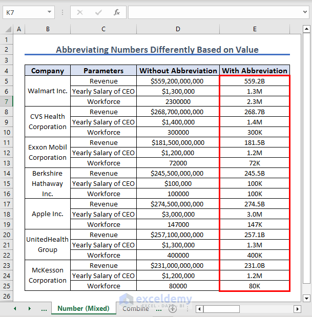
Method 4 – Abbreviating Numbers in Billions, Millions or Thousands

Select E5:E25 >> click Home >> Small Arrow (Number group).
In Format Cells, select Number >> Custom, and enter the following in Type:

[>999999999.999]0.0,,,"B";[>999999.999]0.0,,"M";0,"K"

Click OK.

Copy D5:D25 and paste it in E5:E25.

All numbers are abbreviated.

Read More: How to Abbreviate Numbers in Excel

How to Find a Corresponding Abbreviation from a List in Excel

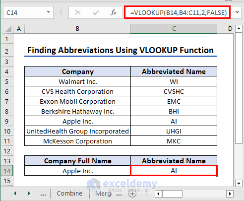
Method 1 – Using the VLOOKUP Function

You have a list of 8 companies with abbreviated names. To find the correct abbreviation, use the VLOOKUP function.

In B14, enter the full name of the company.
Use the following formula in C14:

=VLOOKUP(B14,B4:C11,2,FALSE)

Press ENTER.

You will get the corresponding abbreviated name.

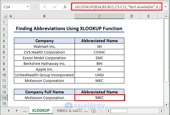
Method 2 – Using the XLOOKUP Function

To find the correct abbreviation for a company name using the XLOOKUP function:

In B14, enter the full name of the company.
Use the following formula in C14:

=XLOOKUP(B14,B5:B11,C5:C11,"Not Available",0,)

Press ENTER.

You will see the abbreviated name. If you enter a name in B14 that is not in the list, the formula returns “Not Available” in C14.

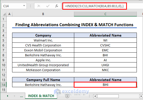
Method 3 – Combining the INDEX & MATCH Functions

In B14, enter the full name of the company.
Use the following formula in C14:

=INDEX(C5:C11,MATCH(B14,B5:B11,0),)

Press ENTER.

You will see the abbreviated name.

Things to Remember

Validate data and ensure the abbreviations accurately represent the original information.
Maintain consistency in your abbreviation approach throughout the spreadsheet or workbook.
Document the abbreviations used, either in a separate key or as a comment within the cell.

Download Practice Workbook

Excel Abbreviation.xlsm

Frequently Asked Questions

1. How do I replace abbreviations in Excel

Answer: To replace an abbreviation in Excel, use the Find and Replace feature:

Select the range that contains the abbreviations you want to remove.
Press Ctrl + H to open the Find and Replace dialog box.
Enter the abbreviation you want to remove in “Find what“.
Enter the content that will replace the abbreviation in “Replace with“.
Click “Replace All“.

2. How do I prevent Excel from abbreviating numbers

Answer: Use an Apostrophe ( ‘ ) before the number.

3. How do I stop Excel from abbreviating dates

Answer: Change the formatting:

Select the cells containing the dates you want to stop Excel from abbreviating.
Right-click the selected cells and choose “Format Cells“.
In “Format Cells“, select “Number“.
Select “Date“.
Choose the a date format.
Click “OK“.

Excel Abbreviation: Knowledge Hub

Use VLOOKUP to Find State Abbreviations

<< Go Back to Learn Excel

Get FREE Advanced Excel Exercises with Solutions!

How to Apply Abbreviation in Excel – Abbreviate Words and Numbers

How to Apply an Abbreviation to an Initial Word in Excel

Method 1 – Combining the LEFT, MID, FIND & LEN Functions to Abbreviate in Excel

Method 2 – Combining the CONCATENATE, LEFT, MID, FIND & LEN Functions

How to Apply Abbreviations to All Words in Excel

Method 1 – Combining the TEXTJOIN, ISNUMBER, MATCH, CODE, MID, ROW, INDIRECT, LEN, and ROW Functions

Method 2 – Combining the UPPER, TRIM, LEFT, MID, FIND, and SUBSTITUTE Functions

Method 3 – Applying a Custom Function Using VBA

How to Abbreviate Days in Excel

Method 1 – Using the TEXT Function

Method 2 – Combining the CHOOSE & WEEKDAY Functions

How to Apply Abbreviation to Numbers in Excel

Method 1 – Abbreviating Numbers in Thousands (K)

Method 2 – Abbreviating Numbers in Millions (M)

Method 3 – Abbreviating Numbers in Billions (B)

Method 4 – Abbreviating Numbers in Billions, Millions or Thousands

How to Find a Corresponding Abbreviation from a List in Excel

Method 1 – Using the VLOOKUP Function

Method 2 – Using the XLOOKUP Function

Method 3 – Combining the INDEX & MATCH Functions

Things to Remember

Frequently Asked Questions

1. How do I replace abbreviations in Excel

2. How do I prevent Excel from abbreviating numbers

3. How do I stop Excel from abbreviating dates

Excel Abbreviation: Knowledge Hub

Leave a reply Cancel reply