How to Abbreviate Numbers in Excel (3 Easy Methods)

Microsoft Excel is a handy software. We use Excel functions and features for our educational, business, and other daily life purposes. Furthermore, Excel provides some cool functions to compress numbers in our workbooks. This article will show you 3 simple methods to abbreviate numbers in Excel.

How to Abbreviate Numbers in Excel: 3 Easy Methods

Handling a long string of numbers in Excel can be really cumbersome. Alternatively, we can easily understand a large number if it is in an abbreviated format. An abbreviated format is a short form of a number or text. A number in its abbreviated form is much easier to understand and read. Moreover, it lessens the chance of errors when we input data in Excel. With that in mind, in this article, I will show 3 easy methods to abbreviate numbers in Excel. For instance, we take a dataset that represents the companies with the highest sales records in a week.

1. Apply Predefined Format to Abbreviate Numbers

Excel provides some useful default number formats to modify our numbers in the dataset. In this article, we will abbreviate large numbers in our dataset using the default Format Cells options. Format Cells options allow us to modify the appearance of a number without tempering its value. The real value appears in the formula bar. But the formatted value will be different in the dataset. This makes the Format Cells option a very useful tool. As we can change our input numbers in different formats, therefore, we can abbreviate large numbers in our dataset using these options. To do so, let’s follow these steps.

Steps:

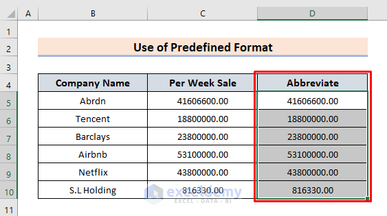
• First, select column D to format it.

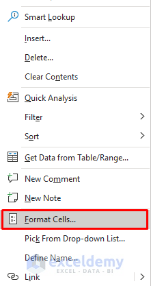
• Next, right-click on the selected range.
• Subsequently, a context menu bar pops up.
• Here, tap the Format Cells option.

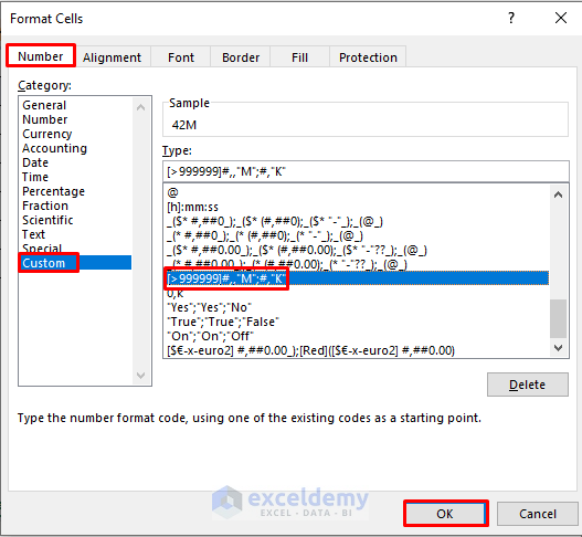
• As a result, the Format Cells options menu opens up.
• Later, select Number then Custom options.
• After that, in the Type box, scroll down to tap [>999999]#,,”M”;#,”K” You can also copy & paste it.

• Finally, hit OK.

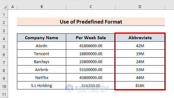
• Thus, the abbreviated number format appears.

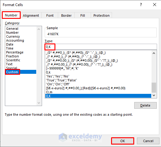
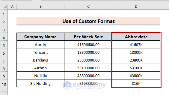
2. Compress Numbers Using Custom Format of Cells in Excel

Similarly, we can abbreviate numbers for better understanding using custom cell formatting. In this case, we can customize our data in any number format we wish. This method also uses Format Cells options like the previous one. The difference is here we customize our own format by typing our custom format options. To illustrate, follow these procedures.

Steps:

• Firstly, Select the desired range you want to format.
• After that, right-click on it and then tap the Format Cells option.

• Consequently, the Format Cells menu will open.
• Here, go to Number > Custom > Type.
• Now, in the Type box, insert the format 0,K.
• Lastly, press OK.

• Hence, we obtain the desired result.

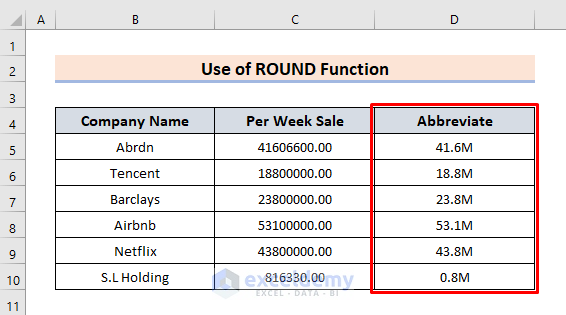
3. Insert ROUND Function to Abbreviate Numbers

To get an abbreviate number format or an approximate value of large numbers, we can implement the Excel ROUND function. The ROUND function returns numeric values in a round or approximate value. It thoroughly makes large numbers more understandable and cleaner. The difference between this method from the previous will be, in this case, the value in the dataset and the one in the formula bar will be similar. The ROUND function tempers the actual data and changes it to the desired formats. This function works in 3 steps. To implement this function, follow the procedures below.

Steps:

• First of all, select cell D5, type the formula,

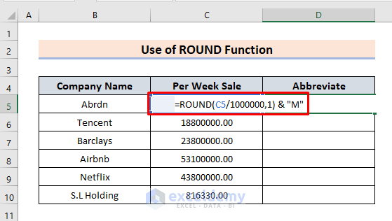
• Next, press Enter and use the autofill feature to fill the other cells.
• Finally, the result pops up in the dataset.

Download Practice Workbook

You can download this workbook to practice yourself.

Conclusion

In conclusion, we have discussed some easy ways to abbreviate numbers in Excel. Please leave any further queries or recommendations in the comment box below.

<< Go Back to Excel Abbreviation | Learn Excel