In this article, we will discuss how to use the VLOOKUP function to find state abbreviations. We often need not the full names but the abbreviations of a state or an organization to do a particular query. Excel offers the VLOOKUP function to address the abbreviations of states or organizations. This will allow users to get the abbreviations easily and use them to do their queries.
How to Use VLOOKUP to Find State Abbreviations in Excel: Step-by-Step Procedures
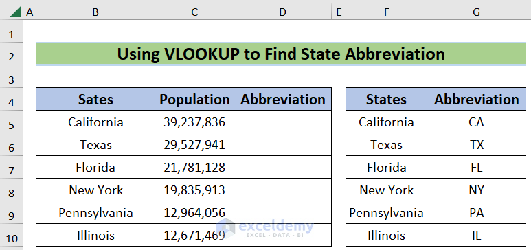
In this article, we will talk about the step-by-step procedure to use VLOOKUP to find the abbreviations of the states of the USA. Here, we have the population data for 6 states of the USA. We will find the abbreviation of the states and put them in the D5:D10 range.
Step 1: Creating Named Range
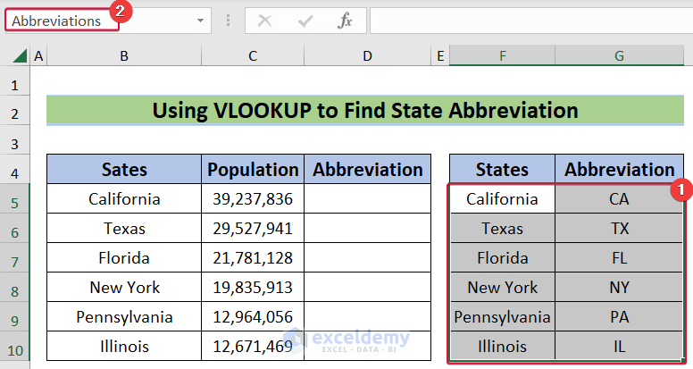
In this step, we will create a Named Range for the states along with their abbreviations. We will name it Abbreviations. The Named Range makes the formula easier to understand.
- Firstly, select the cells in the range F5:G10.
- Secondly, go to the Name Box and type
- Finally, hit Enter.
- As a result, a name will be added to that range.
Step 2: Creating State Abbreviations
In this section, we will type the VLOOKUP formula to enter the abbreviations in the D5:D10 range. The VLOOKUP function takes four arguments. The three required arguments are the lookup_value, table_array, col_index_num. The final argument is optional which asks for the exact or partial match for the lookup value.
- To begin with, click on the D5 cell and enter the following formula,
=VLOOKUP(B5,Abbreviations,2,0)- Then, hit Enter.
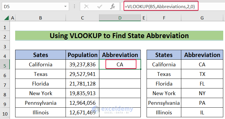
- As a result, we will get the abbreviation of the state of California.
- Finally, lower the cursor down to the last cell to Autofill the cells with the VLOOKUP formula.

This is how we will get the abbreviations of the states of the USA using the VLOOKUP function.
How to Get Full State Name from State Abbreviations
In this method, we will get the full state name from state abbreviations. We will use the combination of the INDEX and MATCH functions to do that.
Steps:
- To begin with, click on the C13 cell and type the following formula,
=INDEX(B5:B10,MATCH(B13,D5:D10,0))- Then, hit Enter.

- As a result, we will get the full form of the state of California.
- Finally, move the cursor down to the last cell to autofill.

Formula Breakdown:
- MATCH(B13,D5:D10,0)): The MATCH function looks for the value in the B13 cell that is CA in the cell range D5:D10 and returns the index number of the cell containing the value. In this case, the value is in the first cell of the D5:D10 range and thus the function returns 1.
- Output: 1
- INDEX(B5:B10,MATCH(B13,D5:D10,0)): This formula turns into INDEX(B5:B10,1). So, the INDEX function looks for the first value in the B5:B10 range which is California and returns it in the C13 cell.
- Output: California
Download Practice Workbook
You can download the practice workbook here.
Conclusion
In this article, we have talked about how to use the VLOOKUP function to find state abbreviations. This method will allow users to find the right abbreviation for the right state and use it in their required field. If you have any questions regarding this essay, feel free to let us know in the comments.
<< Go Back to Excel Abbreviation | Learn Excel
Get FREE Advanced Excel Exercises with Solutions!
