Excel Conditional Formatting with Named Range (3 Examples)

Download Practice Book

Example 1 – Using Array Formula with Named Range in Conditional Formatting

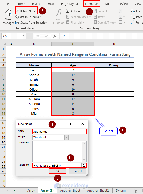
Name the range you want to use inside the conditional formatting formula. Select the range C5:C14 and click on Formulas >> Define Name.

A dialogue box named “New Name” will open. Inside Name:  enter a name. Refers to: is filled by default. Click on OK. The range C5:C14 is now named as Age_Range.

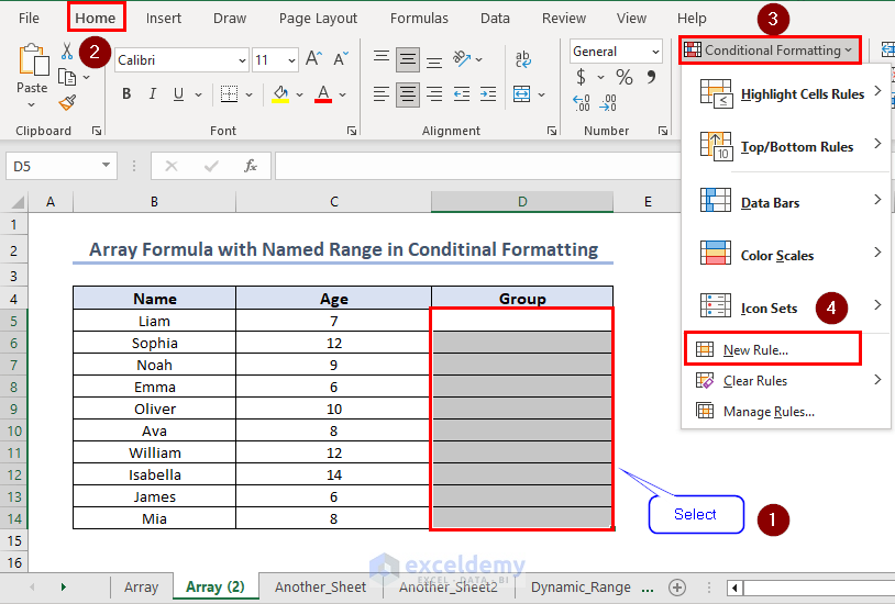
Select the range you want to format and click on Home >> Conditional Formatting >> New Rule…

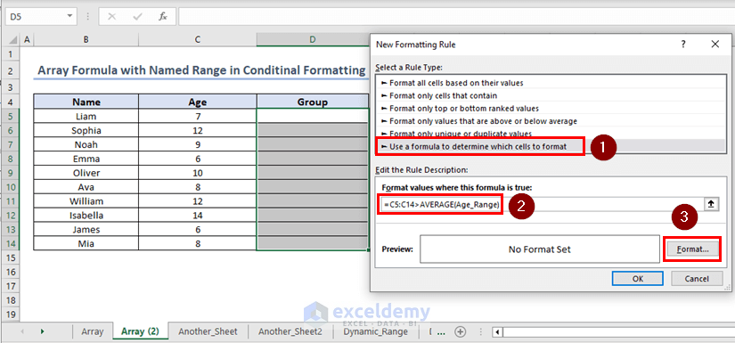
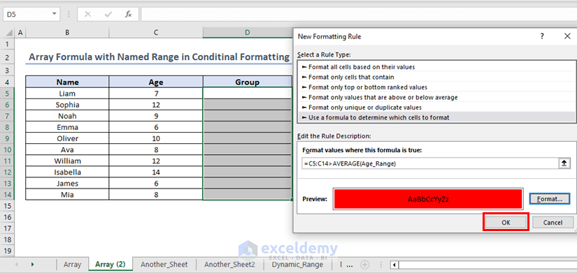
Inside the dialogue box named “New Formatting Rule” select Use a formula to determine which cells to format. Under Format values where this formula is true:, enter the following formula:

(which is an array formula as it takes array C15:C14 as an input)

Click on Format.

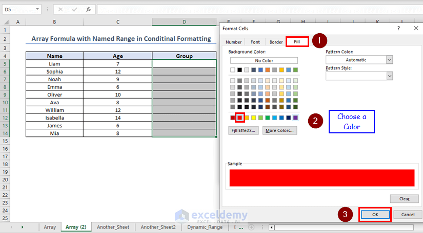
A dialogue box named “Format Cells” will open. Under the Fill tab, choose any appropriate color and click on OK.

Inside “New Formatting Rule” click on OK.

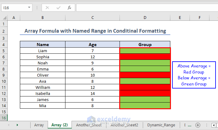
This will format the cells corresponding to the children whose ages are greater than the average age with red fill.

To highlight cells, corresponding to those whose ages are below the average age, follow the same procedure with a modified formula given below

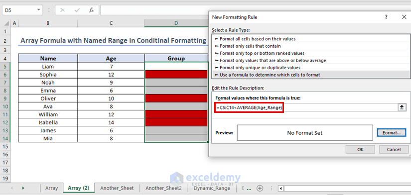
Children whose ages are higher than the average age are in the red group and those whose ages are less than the average age are in the green group.

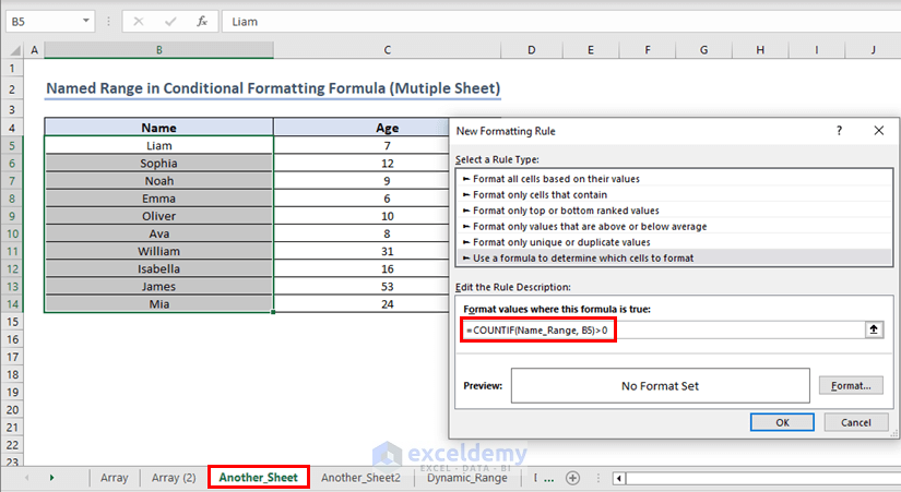
Example 2 – Using Conditional Formatting with Named Range on Another Sheet

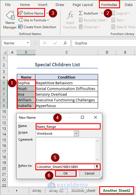
Inside the sheet named “Another_Sheet2”, select the range B5:B9 and click on Formulas >> Define Name. Enter a name. The Refers to: is filled by default. Click on OK.

Go to the sheet named “Another_Sheet” and create a new conditional formatting rule. Enter the following formula below:

Assign formatting.

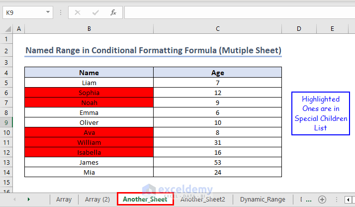
This action will highlight the names in “Another_Sheet”, which are also available inside the range named “Name_Range” inside the “Another Sheet2” sheet.

Example 3 – Conditional Formatting with Dynamic Named Range

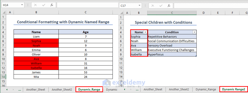
To make the outcome of example 2 dynamic, convert the dataset in sheet “Dynamic_Range2” into an Excel table.

Select the Range B4:C9 and press CTRL+T. Inside the “Create Table” dialogue box, click on OK.

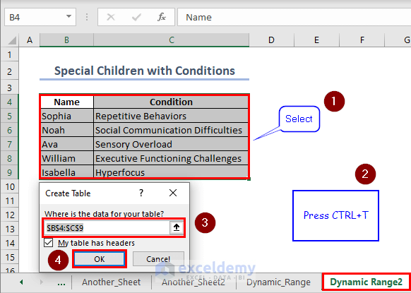
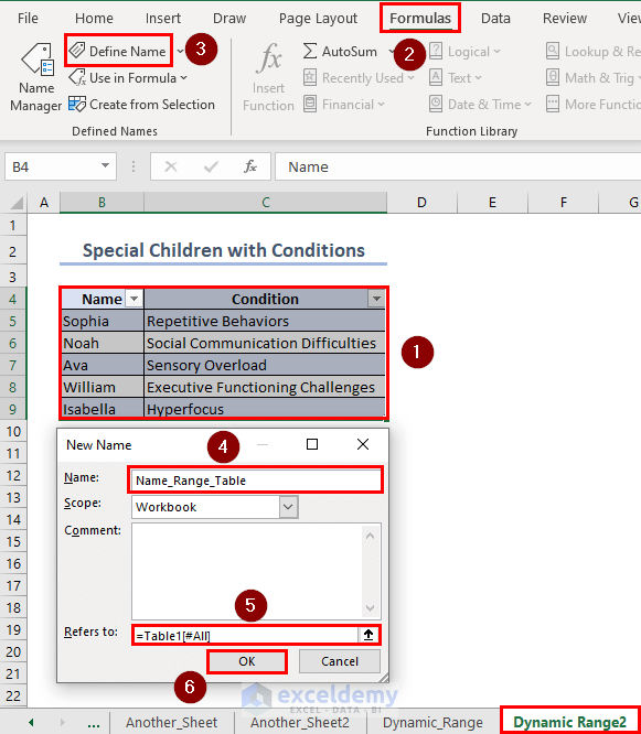
The selected range will convert into an Excel table. Name the table. We have named it “Name_Range_Table”.

Go to sheet “Dynamic_Range” and insert a new formatting rule for range B5:B14 using the following formula below,

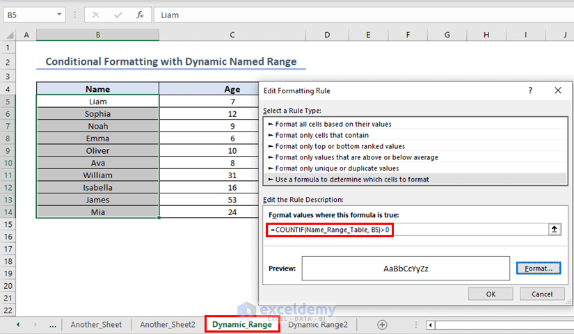
The names in sheet “Dynamic_Range” which are also present inside the table in sheet “Dynamic_Range2” are highlighted.

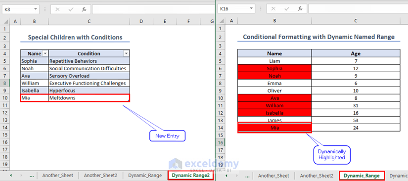
To test if the output is dynamic or not, enter a new name inside the table in sheet “Dynamic_Range2” and observe that the same name in sheet “Dynamic_Range” is highlighted.

Things to Remember

• Make sure you correctly define the named range to include the desired cells. The named range should be appropriate for your specific data, and it should not include any unnecessary cells or exclude relevant ones.
• In the case of new naming, avoid the name that is already present in the same workbook.
• The order of the conditional formatting rules matters. Excel applies rules from top to bottom. Make sure to arrange the rules in the desired priority so that the formatting you want takes precedence.

Frequently Asked Questions

• What happens if I modify or delete the named range used in conditional formatting?

If you modify or delete the named range, the conditional formatting rule will lose its reference, and the formatting may not be applied as intended.

• Can I use multiple named ranges in a single conditional formatting rule?

Yes, you can use multiple named ranges in a single conditional formatting rule by incorporating them into the formula as needed.