How to Use Named Range in Excel VLOOKUP Function

The VLOOKUP function is one of the most commonly used functions in Microsoft Excel. We use the VLOOKUP function to find values in a table to extract its corresponding information. Sometimes we need to select a range of cells to refer to but we end up selecting incorrect ranges that make things complicated for us. In these types of cases, we can use the named range with the VLOOKUP function to create references and use this in our formulas. The purpose of this article is to explain the Excel VLOOKUP function named range in order to reference data.

 How to Use VLOOKUP Function with Named Ranges in Excel: 2 Easy Ways

To show the VLOOKUP function with named range, we have taken a brief dataset that contains 11 rows and 5 columns of Order ID, Rep Name, Item, Units and Unit Cost. Applying named ranges in the VLOOKUP function enables us to simplify the formula. We can use that named range as a reference in formulas. For this article, we are going to use Excel 365 version. You can use any other version of Excel as well.

1. Using Excel VLOOKUP Function with Named Range

The VLOOKUP function is applied when we need some information from a dataset and want to extract its corresponding value. On the other hand, named range is a group of cells or values that is given a name so that we can access those cells in our formulas by only using that range or reference name. Using the named range in the VLOOKUP function makes formulas easier and simpler to understand. If you want to get a clear understanding, go through the following steps.

First, I will show you how to create a named range of our selected dataset. Suppose we want to create a named range or reference of column Rep Name, Item, and Units which are columns C, D and E respectively. Go through the below steps.

Steps:

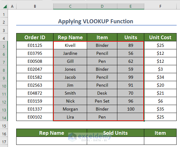
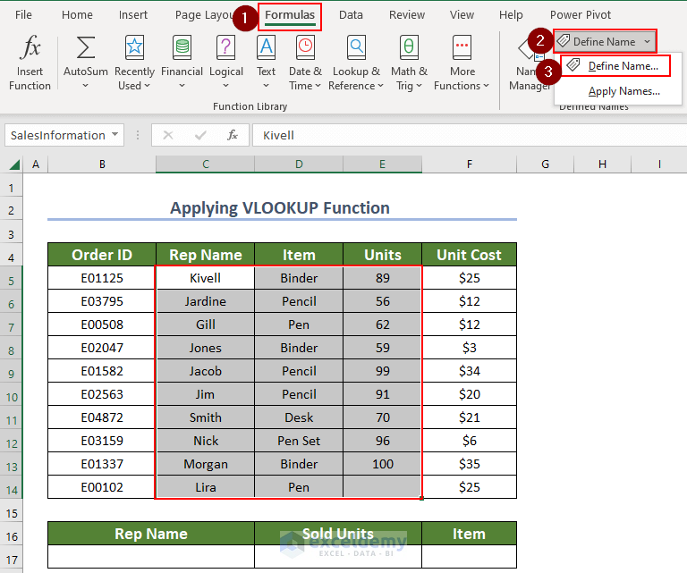
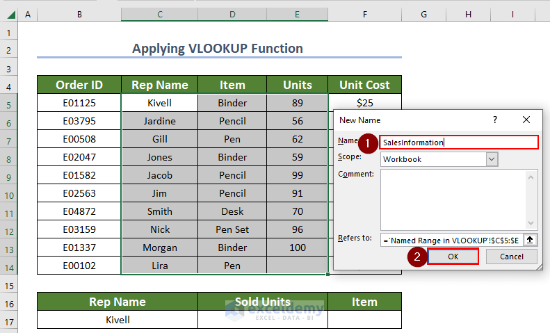
• First, select the range that you want to give a name. In this dataset, C5:E14 is the range that we want to give a specific name.

• After that, right-click on your mouse and select Define Name.

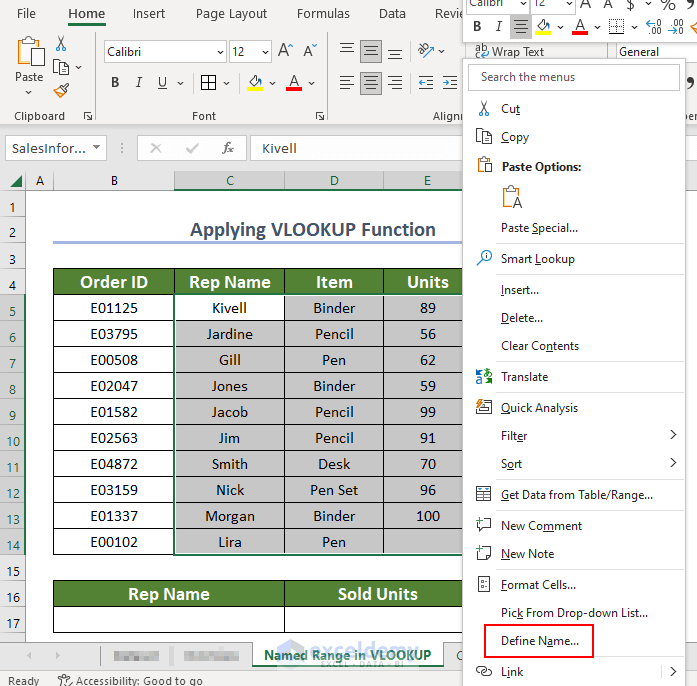
• As a result, a New Name tab will be popped up.
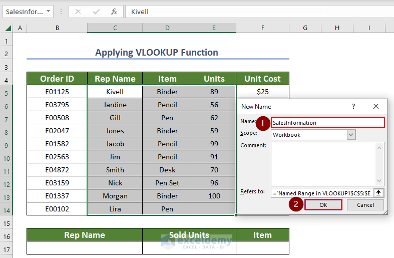
• Then, type your preferred reference name in the Name field. SalesInformation is the reference name in our case.
• Finally, click OK.

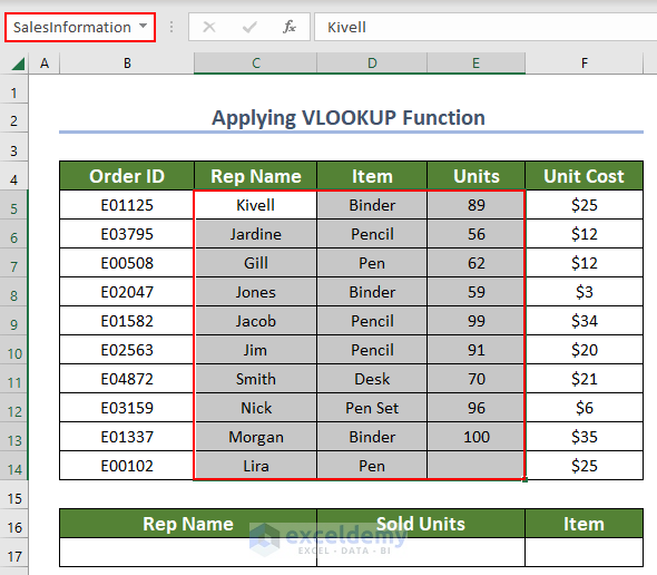
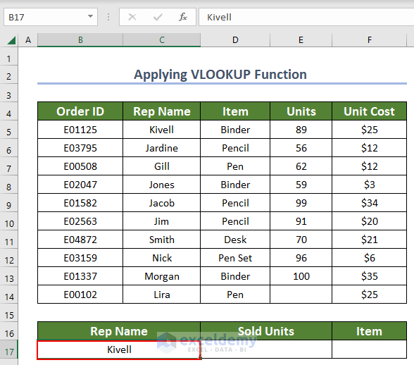
Finally, if we select our range we can see the name of the range in the Name Box and that is SalesInformation.

You can create a named range in another way. To do so follow the below steps.

• First, select the range (C5:E14) that you want to give a name.
• Then, go to the Formulas tab and click on Define Name dropdown.
• After that, select Define Name.

Therefore, it will take you to the same exact New Name screen where you can define your reference name and create a named range.

Moreover, I will show you how to use this created named range in the VLOOKUP function. Suppose we want to find out Kivell’s information which is selling items and units. Let’s go through the following steps.

• First, select cell B17:C17 to enter the Rep Name.

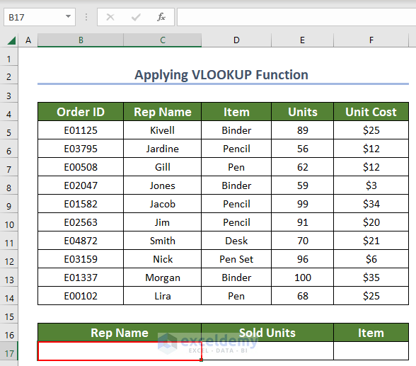
• Furthermore, enter the Rep Name in cells B17:C17.

• After that, select cells D17:E17 to enter the VLOOKUP formula.

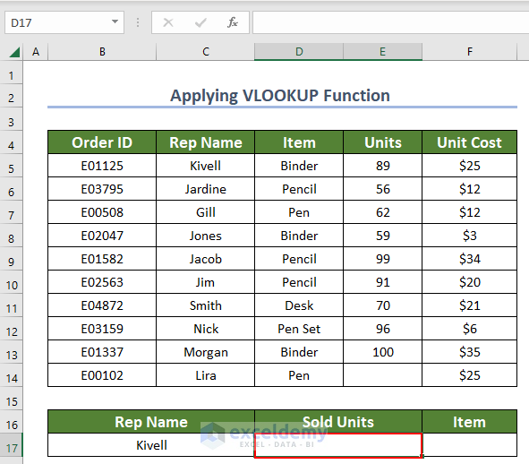
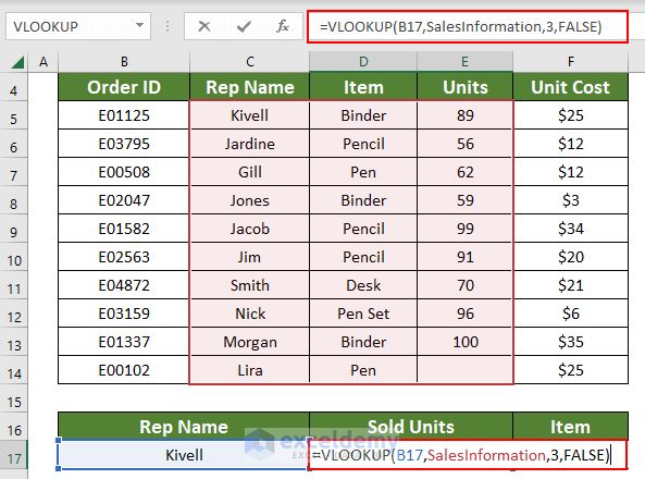
• After that, insert the following formula in cells D17:E17 to apply the VLOOKUP formula using the named range.

 Here, SalesInformation is the named range that is previously created.

• Finally, press the ENTER The output will be shown in cells D17:E17.

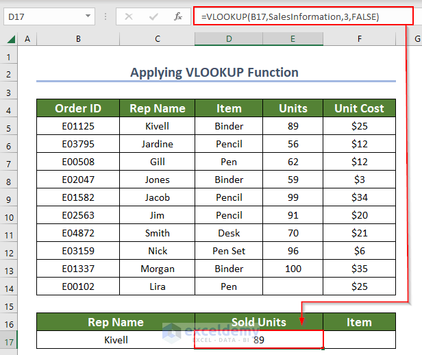
Here, we got the Sold Units of Kivell. We just used the created named range in the VLOOKUP function and it gave us the required information. This is the benefit of using named range in the VLOOKUP function.

You can also get the Item by applying the same formula with a little bit of change. Let’s go down the below part of this article.

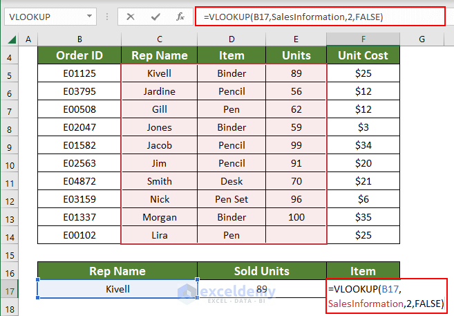
• First, select cell F17 to apply the formula.

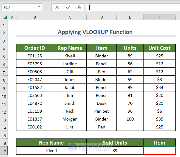
• Thereafter, insert the following formula in cell F17 to apply the VLOOKUP formula using the named range.

 Here, SalesInformation is the named range that was previously used. The only change in this formula is we have given 2 as a col_index_num since the column index number of the Item column is 2.

• Finally, press ENTER.  The output will be shown in cell F17.

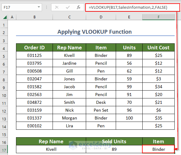
Here, we got the Item associated with Kivell which is Binder. So in this way, we can easily create a named range and use this named range as a reference in our formulas to get the value.

Read More: Excel Reference Named Range in Another Sheet

2. Applying Named Range with VLOOKUP Function for Multiple Sheets

In this method, I will explain how to use the Excel VLOOKUP function with a named range across multiple sheets. We will use the IFNA, INDIRECT, INDEX, MATCH, and COUNTIF functions along with the VLOOKUP function to do the task. Suppose we have multiple sheets and we want to apply the VLOOKUP function at a time with a named range.

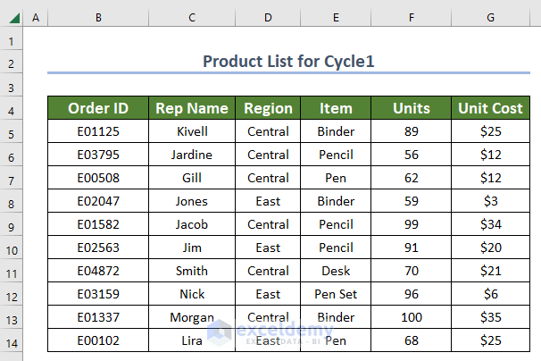
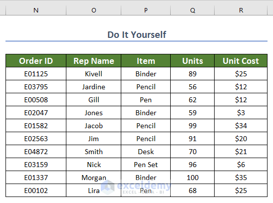
We have two different sheets named Cycle1 and Cycle2. Both have 11 rows and 6 columns named Order ID, Rep Name, Region, Item, Units and Unit Cost.

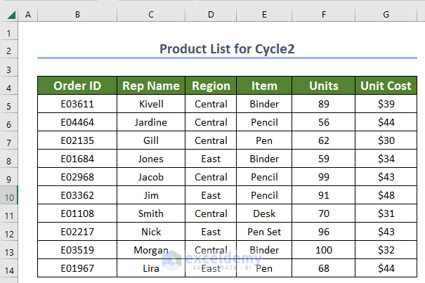
The Cycle2 sheet contains the same number of rows and columns.

We have another sheet named Multiple Sheet, where we will apply our formula. After that, let’s carry out the following steps.

Steps:

• First of all, select cells B8 and B9 to write down all the lookup sheet names.

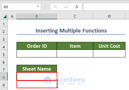
• Then, write down lookup sheet names which are Cycle1 and Cycle2.

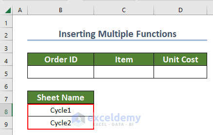
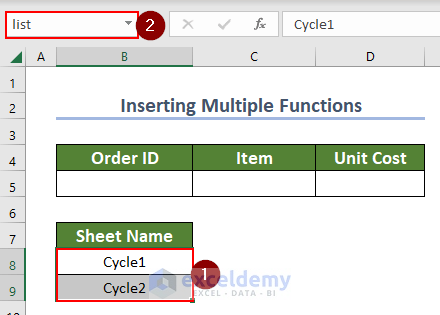
• Afterward, select Cycle1 and drag your cursor to select Cycle2.
• After that, type your preferred reference name in the Name Box( list in our case).

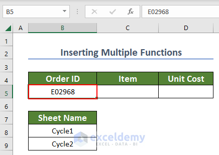
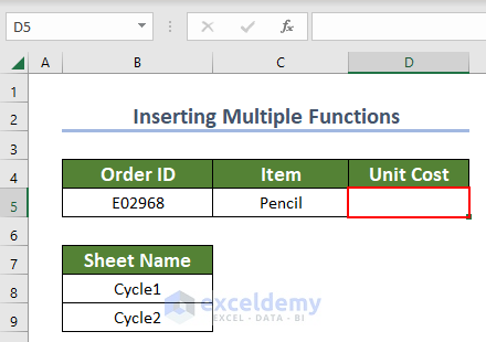
• In addition, select cell B5 to enter the Order ID.

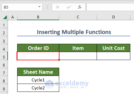
• Following this, enter your preferred Order ID (E02968).

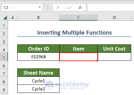
• Moreover, select cell C5 to enter the VLOOKUP formula.

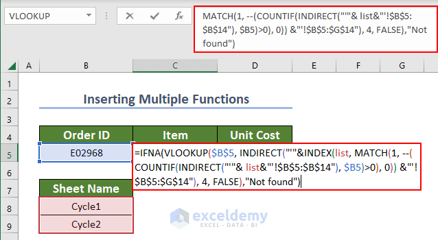
• At this point, insert the following formula in cell C5 to apply the VLOOKUP formula using the named range.

 Here, the list is the named range of lookup sheets Cycle1 and Cycle2.

• Finally, press ENTER The output will be shown in cell C5.

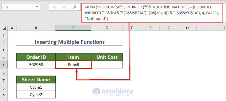
Therefore, we got the output in cell C5 which is the Item ‘Pencil’ corresponding to Order ID E02968 from the Cycle2 sheet. We could easily do that by applying named ranges in the VLOOKUP function.

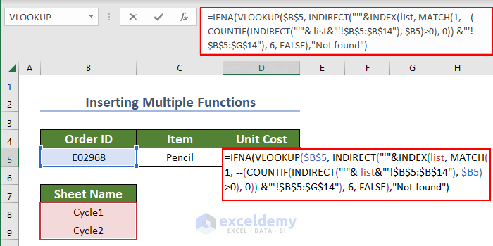
After that, you can also find the Unit Cost corresponding to Order ID E02968 by applying the same formula with a little bit of change. To do so carry out the below steps.

• First, select cell D5 to enter the VLOOKUP formula.

• After that, insert the following formula in cell D5 to apply the VLOOKUP formula using the named range.

 The only change in this formula is, here we have put 6 for column index number for column Unit Cost.

• Then, press ENTER The output will be shown in cell D5.

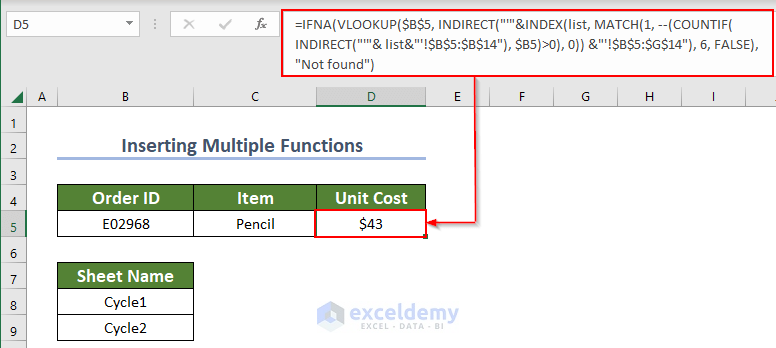
Here, we got the output in cell D5 which is the Unit Cost ‘$43’ corresponding to Order ID E02968 from Cycle2 sheet. So, in this way, we can retrieve the corresponding item from multiple sheets using the VLOOKUP function with name ranges. It makes calculation easier and quicker.

Read More: Excel INDIRECT Function with Named Range

Practice Section

You can use the following dataset to practice by yourself. You can modify it too if it is necessary. Hope it will help you to practice how to use the named range in the VLOOKUP function effectively.

Download Practice Workbook

You can download the practice workbook from here:

Conclusion

In this article, I tried my utter level best to show you how to use Excel VLOOKUP Function with named range across multiple sheets and retrieve corresponding information. I hope this article will be helpful for you to solve these types of problems. You have any suggestions and query leave a comment below.

Related Articles

• How to Ignore Blank Cells in Named Range in Excel
• How to Create Dynamic Named Range in Excel
• How to Use Dynamic Named Range in an Excel Chart
• Define Names with the Create from Selection Tool in Excel

<< Go Back to Named Range | Excel Formulas | Learn Excel