Excel Named Range (A Complete Guideline)

Excel named range allows users to assign names to specific cells or ranges. This feature increases clarity and efficiency while working with large datasets.

In this tutorial, you will learn about Excel named ranges, including their creation, applications, and advantages.

In the example below, we created a named range using the Name Box in Excel.

In this blog post, you will learn-

– What is Named Range and why use it?
– Naming rules for Named Range
– To create Excel Named Range
– To create Dynamic Named Range
– To Find, Edit, Filter and Delete Named Ranges
– To define names for formulas
– Issues with Named Ranges

Named range is available from the Excel 2007 version. Here, I have used the Microsoft 365 version of Excel to make this article.

⏷What Does “Name” Mean in Excel?
⏷What Is Named Range in Excel?
⏷Why Use and When Not to Use Named Ranges?
⏷How Many Named Ranges Can We Create?
⏷Naming Rules for Named Ranges
⏷Create Named Range in Excel
    ⏵Using Name Box
    ⏵Using Define Name Option
    ⏵Using Name Manager
    ⏵Using Create from Selection 
⏷Create Dynamic Named Range in Excel
    ⏵Using Excel Tables
    ⏵Applying Formulas
⏷Find Named Ranges
⏷Keyboard Shortcuts for Named Range
⏷Edit, Filter and Delete Named Ranges
⏷Get List of All Named Ranges in Workbook
⏷Ignore Blank Cells in Excel Named Range 
⏷Dynamic Named Range in Excel Chart 
⏷Tips and Tricks for Named Range 
⏷Create Name for a Constant in Excel
⏷Define Name for a Formula in Excel 
⏷Name Columns and Rows in Excel
⏷Use Named Range in Another Sheet
⏷Issues with Named Ranges in Excel

What Does the Term “Name” Mean in Excel?

In Excel, the term “Name” means meaningful and usable names of range or cell.

For example, in the following formula, we enter the reference of cells containing marks to calculate their sum.

We can define the cell references as marks and enter this name instead of cell references to make the formula easier to read.

Name Types in Excel

In Excel, there are two types of Names.

Defined Names: When you give a name to a single cell, group of cells, formula, or constant value, those are defined names.

Table Names: Excel automatically gives names to cell ranges when creating a table, and these names are called table names.

What Is Named Range in Excel?

Excel’s named range feature allows you to assign a meaningful name to a specific cell or range of cells. In functions and formulas, you can use this name instead of cell references (like you can name the range F6:F15 as Annual_Salary).

Why Use Named Ranges in Excel? When Not to Use It?

Below, we have discussed the reasons for using Named Ranges.

• Named ranges are easier to navigate. You can type any name in the Name Box, and Excel will immediately select the name range in the spreadsheet.
• You do not have to select the cell ranges manually every time.
• Named ranges can be managed easily in Name Manager.
• Named ranges make complex formulas with a lot of referencing more understandable.
• Dynamic named ranges allow you to make the formulas dynamic too.
• By naming a formula, you can use it multiple times without typing the formula every time. You just have to type the name to access the formula.
• You can make a drop-down list easily.

In some cases, creating a large number of named ranges and using them in loops in the worksheet might slow down your Excel. That might hamper your workflow.

What Are the Naming Rules for Excel Named Range?

In Excel Named Range, no name should exceed 255 characters. There are also some rules for naming an Excel Named Range:

• Names in Excel must begin with a letter, underscore (_), or backslash (). Any other character is not allowed as the first character of the name.
• Letters, underscores, periods, and numbers can be used as the remaining characters of the name.
• Excel names don’t care about cases of text. For example, “Sales,” “sales,” and “SALES” are considered the same name.
• Space characters are not allowed to be used in names.
• It’s not possible to name a range in the same way as a cell reference. You can’t give a range the name “B1” or “AZ1”. However, you can name a range with a single letter such as “a”, “b”, “D”, and so on, except for the letters “r”, “R”, “c”, and “C”. These letters are shortcuts that allow you to select a row or column for the currently selected cell.

How Many Named Ranges Can We Create in Excel?

Microsoft does not specify the maximum number of Named Ranges you can have. At 32,768 Named Ranges, Excel might stop functioning correctly. Some advanced users have discovered that Microsoft Excel can handle named ranges of 32,768 to 65,536.

How to Create Named Range in Excel: 4 Suitable Ways

In this section, we will demonstrate 4 suitable ways of creating a named range in Excel.

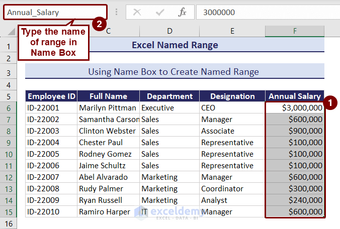
1. Create Named Range Using Name Box

From our dataset, we will create a name for the Annual Salary column using the Name Box.

• For that, select the cell range F6:F15 >> go to Name Box >> type “Annual_Salary” and press Enter.

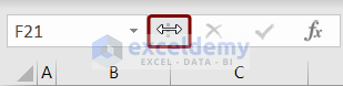
Resize Name Box:

In Newer Excel versions, you can resize the name box if it seems small. In the previous version of Excel, this option was not available. Name boxes used to be only of a definite size.

• Hover the cursor to the three vertical dots beside the Name box.
• The mouse pointer will change to a two-sided arrow.
• Now, drag it to the right or left to increase or decrease the size of the Name Box.

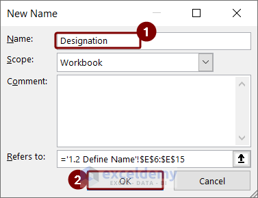
2. Using Define Name Option

In this method, we will create a name for the Designation column using the Define Name option.

• Select the cell range E6:E15 >> go to the Formulas tab >> from the Defined Names group, select Define Name.

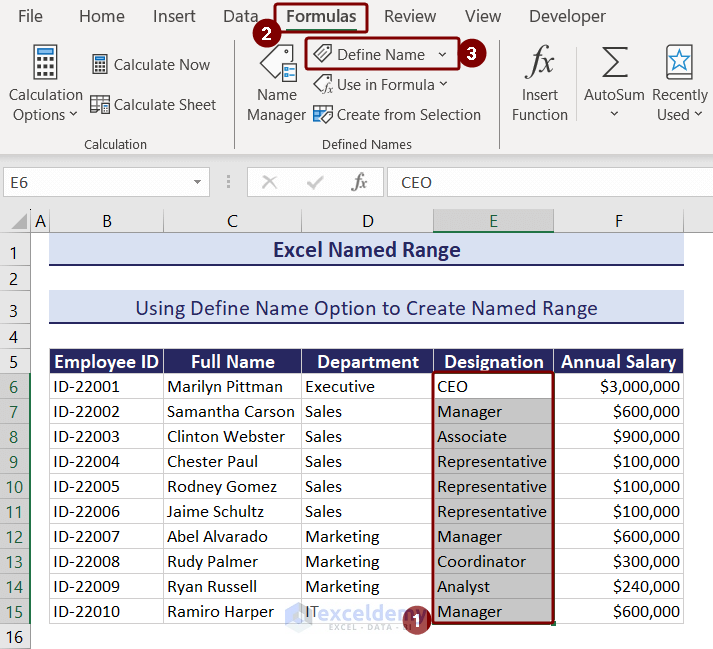
A dialog box named New Name will appear.

• Type “Designation” in the Name box >> keep the Scope as Workbook.
• You can add any comment about the name created in the Comment box. Here, we did not add any comments, so we kept it blank.
• Next, in the Refers to box, you can see the reference to the selected cell range >> press OK.

How to Change Scope of Named in Excel

Scope determines where named ranges can be used. There are two levels of scope in Excel.

Workbook scope: any sheet of any workbook.

Sheet scope: only within that sheet.

Now, we will change the Scope named range “Designation” using the Define Name option.

But You Can’t Change Scope After Creating a Named Range.

First, we will show you that:

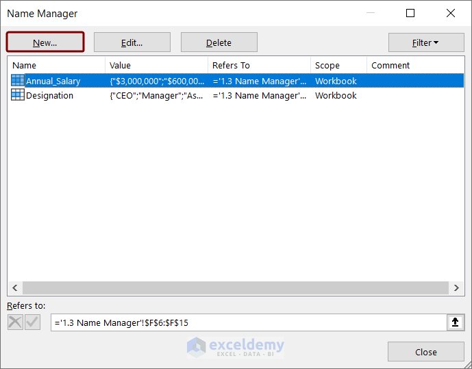
• Select Name Manager from the Formulas tab.

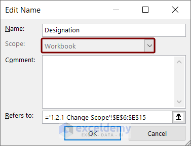
• Then, select “Designation” named range >> click on the Edit option.

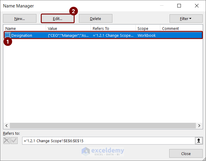
You can see that the Scope box is grayed out in the Edit Name box. Thus, you cannot avail of the option to change the scope.

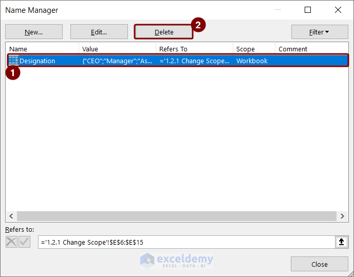
Since we cannot change the scope after defining the name, we will delete this defined name and define a new named range with a different scope.

• Open the Name Manager >> select the “Designation” name, and click the Delete option >> press OK.

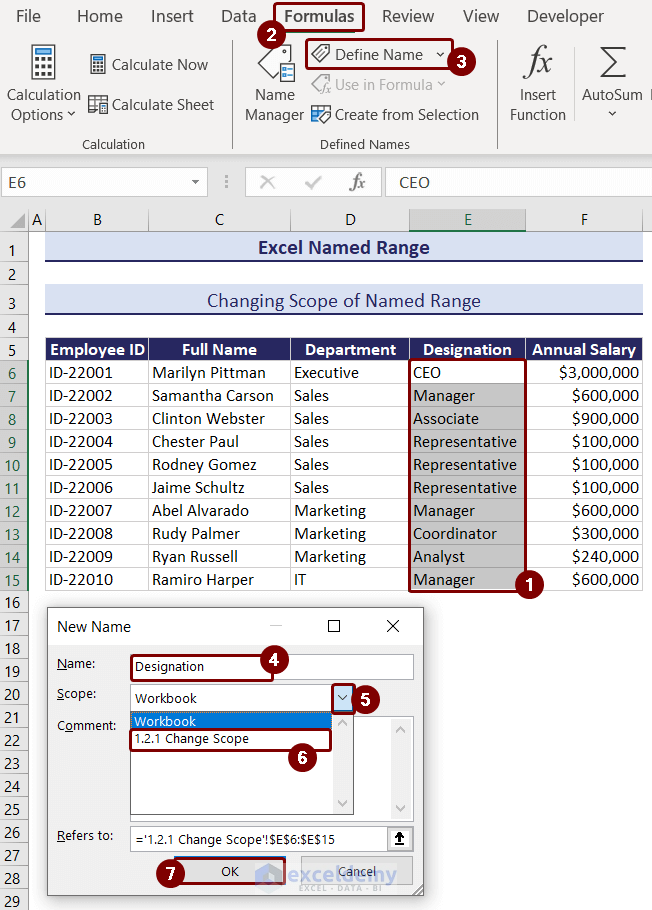
Now, to define a name with a different scope,

• Select the cell ranges E6:E15 and click Formulas >> Define Name.
• In the New Name box, type “Designation”.
• Click on the drop-down of the Scope box, and select the Sheet Name from the list.
• In the Refers to box, you can see the selected cell range; recheck that and press OK.

3. Using Name Manager

We will name the ‘Department’ column using Name Manager.

• Click the Formulas tab >> Name Manager option.

• In the Name Manager dialog box, click New.

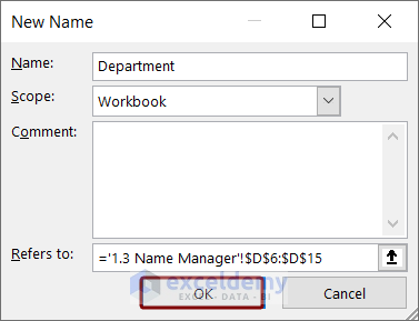
• Type a name in the Name box. We typed Department.
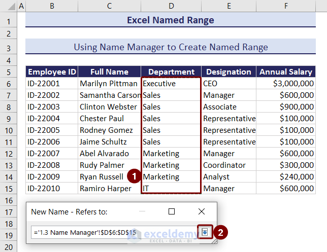
• Then, click the upside arrow beside Refers to box.

• Next, select the cell range. We selected D6:D15, the cell range of the department column.
• After selecting, click on the downward arrow in the New Name- Refers to dialog box.

• Now you can see the cell reference of the selected range in the New Name dialog box, and press OK.

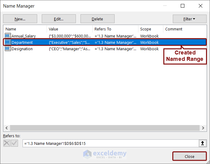
• Next, the Name Manager box will show up, viewing the created named range “Department”. Press Close there.

4. Using Create Selection Option

We will name the employee’s Full Name column using Excel’s Create from Selection tool.

• Select the range C5:C15, where C5 contains the column header (Full Name).
• Go to the Formulas tab.
• Click on the Create from Selection option from the Defined Names group.

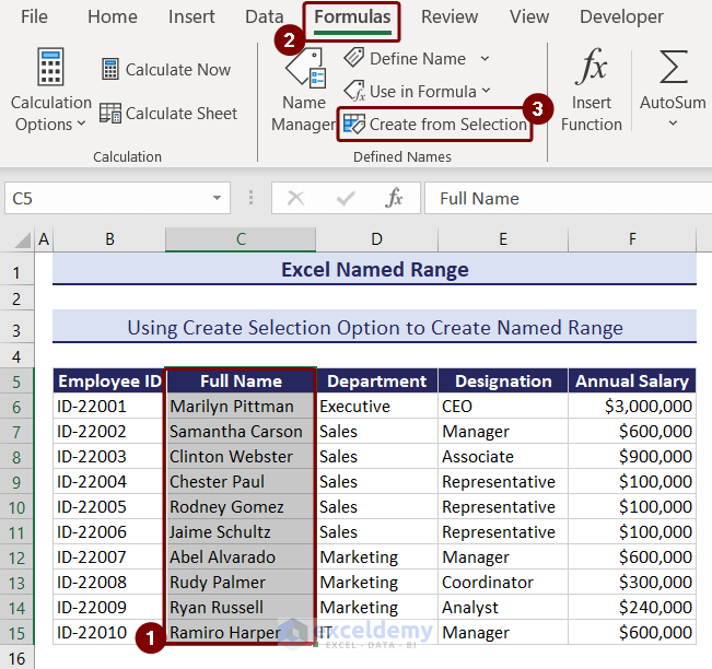
• A dialog box named Create Names from Selection will appear.
• Select the Top row from the options and press OK.

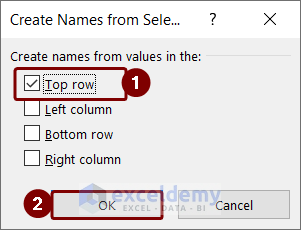
The named range will be created. Since we selected the Top Row option, the range’s name will be Full Name according to the dataset. You can check it in the Name Manager.

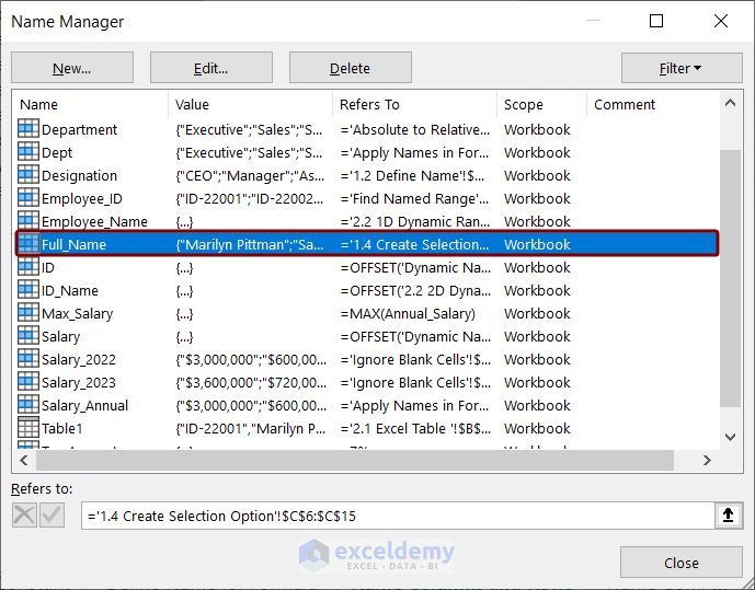
Here, the created named range has a workbook-level scope. So, the named range you create in this way is valid for all other named ranges in the workbook.

How to Create Dynamic Named Range in Excel: 2 Useful Ways

Static named ranges do not expand with new data entry, while dynamic named ranges expand automatically. You can create a dynamic named range using a table or by applying the formula in Excel.

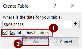
1. Use Excel Tables to Create a Dynamic Named Range

We will create the table from the whole dataset to create a dynamic named range.

• First, select the cell range B5:F15.
• Click the Insert tab >> Table option from the Tables group.

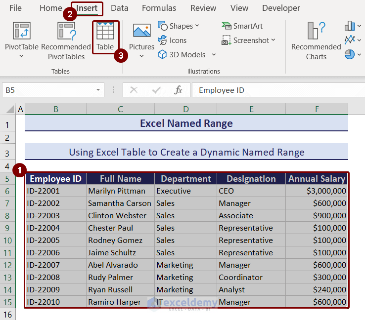
• A box named Create Table will appear, where you will see the reference of the selected cell.
• Check the box My table has headers as the selected range has headers.
• Press OK.

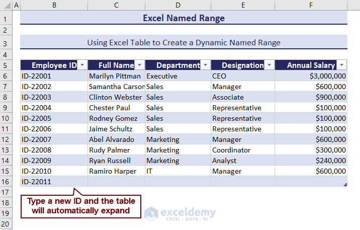
Now, let us check if it has become dynamic or not. We typed a new ID under the last ID entry, and the table expanded automatically.

2. Apply Formula to Create Dynamic Range

You can create one or two-dimensional dynamic named ranges by applying the formula.

1. One-Dimensional Dynamic Named Range

From our dataset, we will create a one-dimensional dynamic named range for the Full Name column.

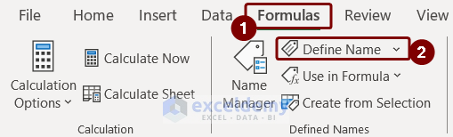
• Click on the Formulas tab > Define Name.

• In the New Name box, type Employee_Name.
• Next, in the Refers to box, enter the following formula and press OK.

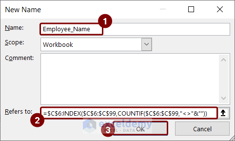
• Select any cell and type the named range, and you will see the contents of the dynamic named range.

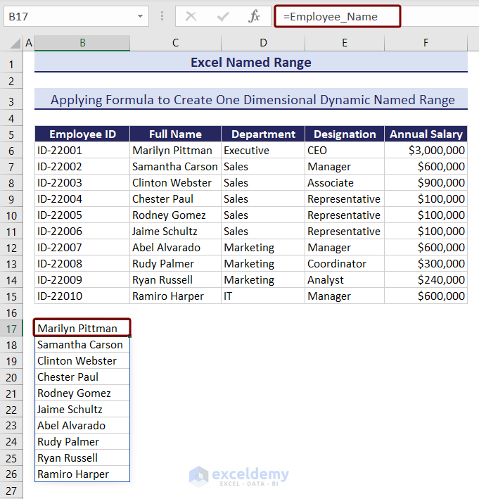
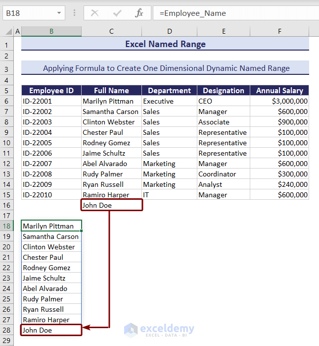
Now, we entered a new name under the Full Name column. You can see the name automatically added in the dynamic named range below.

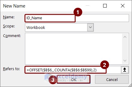
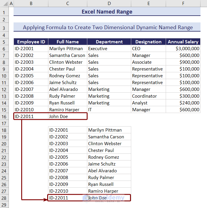
2. Two-Dimensional Dynamic Named Range

Now, we will make a two-dimensional dynamic named range using OFFSET and INDIRECT functions. We will name the ID and Name columns together.

• Go to Formulas > Define Name.

• In the New Name box, type ID_Name.
• Now, enter the following formula in the Refers to box.

Or

• Press OK.

• In cell C17, type the named range we created just now

And you can see the two-dimensional dynamic named range visible there.

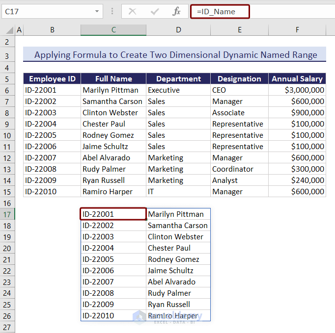
Now, we entered a new ID and name under the Employee ID and Full Name column. You can see the name automatically added in the dynamic named range below.

How to Find Named Ranges in Excel

We can find the named ranges in Excel using the Go To feature. For example, we want to find the named range ‘Employee_ID’.

• Go to the Home tab >> expand Find & Select option >> Go To option.

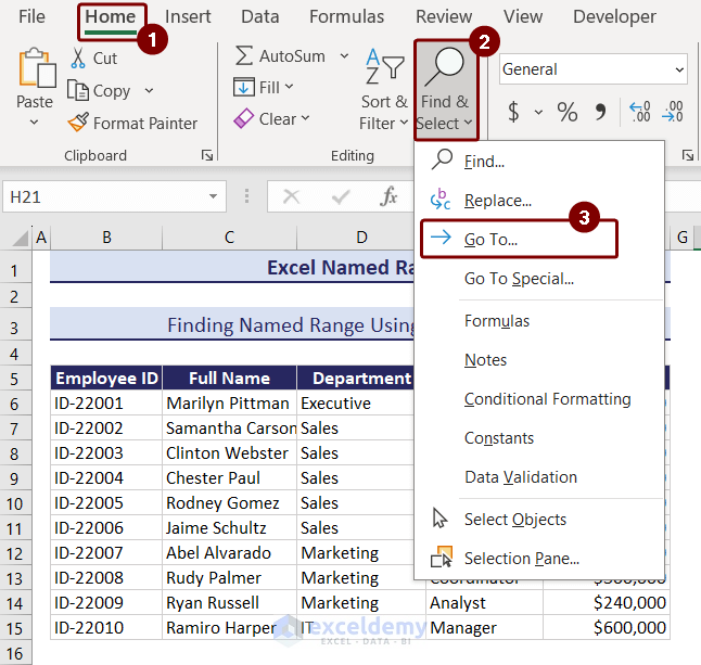
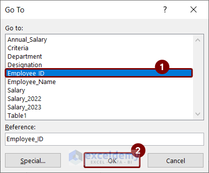
• A box named Go To, with a list of named ranges, will appear.
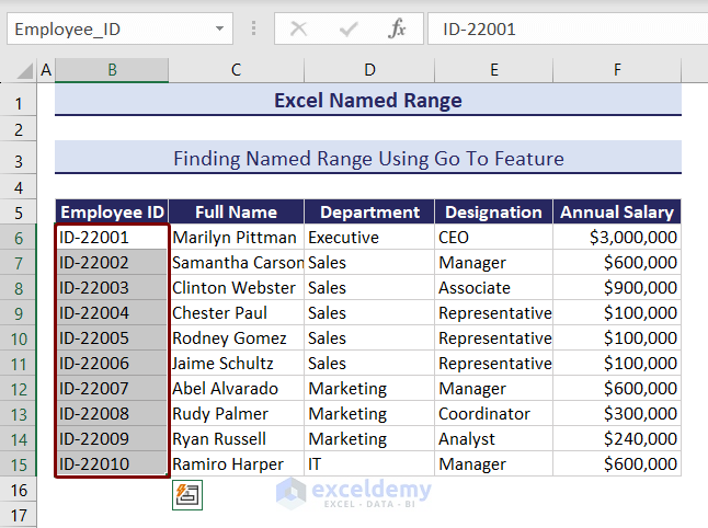
• Select Employee_ID named range >> press OK.

You will see the named range selected in your dataset.

What Are the Keyboard Shortcuts for Excel Named Range?

There are some keyboard shortcuts for creating named ranges in Excel.

• Ctrl + Shift + F3: To avail Create from selection option.
• Ctrl + F3: To open Name Manager in Excel.
• F3: To get the list of all Excel names created in a workbook.

How to Edit, Filter and Delete Named Ranges in Excel

Using Name Manager we can edit, filter, and delete named ranges in Excel. Let us show you how to do that.

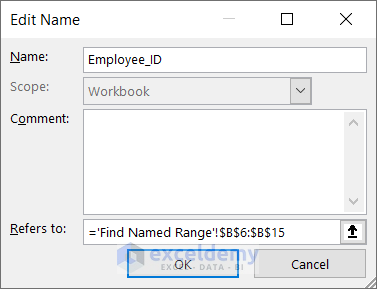
1. To Edit Named Ranges in Excel

Using the Name Manager, we can edit named ranges in Excel. Here, we want to edit the named range “Employee_ID” which we have already created.

• Select the Formulas tab > Name Manager.

• In the Name Manager dialog box, select the Employee_ID named range.
• Press the Edit button.

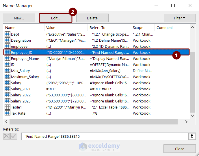
• A box named Edit Name will pop up.
• Now, you can change the name of the named range in the Name field.
• You can change the cell references in the Refers to box. You can either type the cell reference or click the upside arrow and select the cell range directly from your dataset.
• Press OK to save the changes.

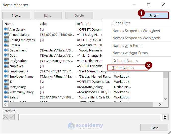
2. To Filter Named Ranges in Excel

Using Name Manager, you can also filter the names. There are different filtering options, such as:

– Clear Filter
– Names Scoped to Worksheet
– Names Scoped to Workbook
– Names with Errors
– Names without Errors
– Defined Names
– Table Names

We will filter table names from the name list.

• Open the Name Manager from the Formulas tab.
• Click on the Filter option.
• Choose Table Names to filter out the tables.

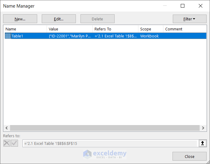
• Name Manager will show the table name that we created while demonstrating the way of creating a dynamic named range.

3. To Delete Named Ranges in Excel

In this section, we will delete the named range “Count Employees” using Name Manager.

• Open Name Manager.
• Select the name “Count Employees”.
• Press the Delete button.

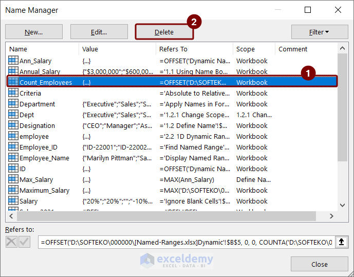
• A warning message will appear. Press OK to delete the named range.

Read More: How to Delete All Named Ranges in Excel

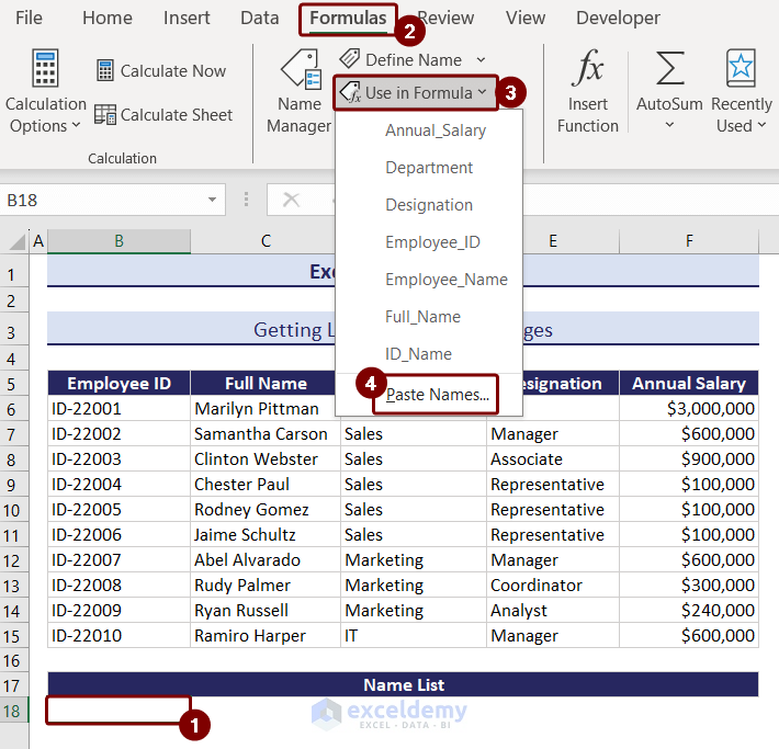
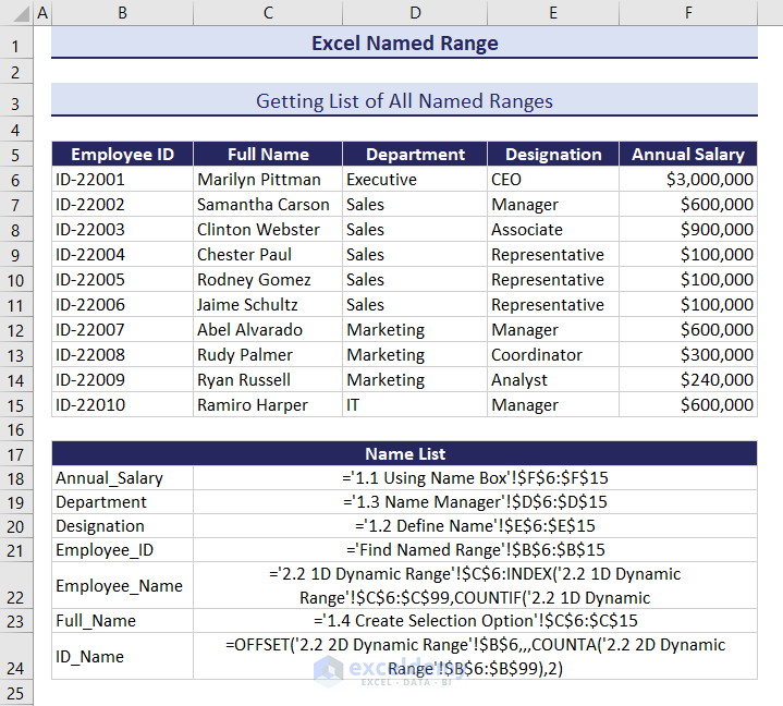
How to Get List of All Named Ranges in Workbook

To avoid forgetting named ranges, Excel allows you to paste the range list in the spreadsheet with the cell reference of the data.

We will paste all the named ranges listed in our dataset.

• First, select cell B18.
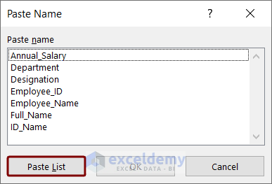
• Next, go to the Formulas tab >> Use in Formula >> Paste Names.

• Paste Name box with the name list will be visible.
• Click on the Paste List option to get the list.

• Lastly, you will see the named ranges with their data references in the selected cell.

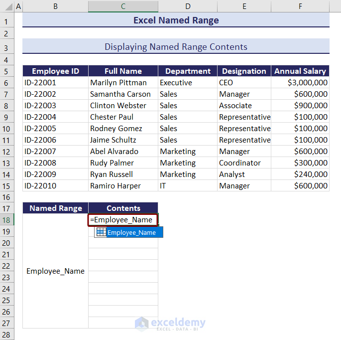
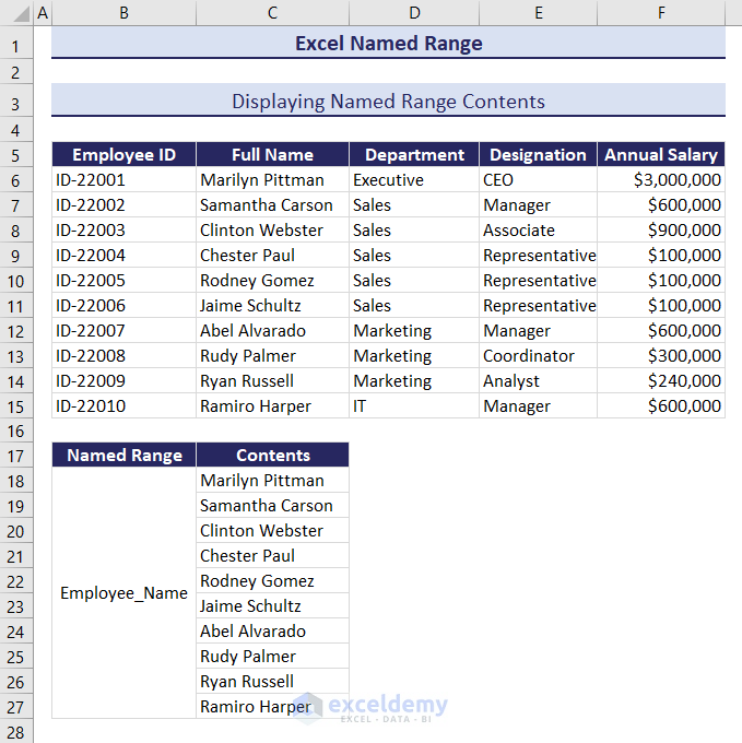
How to Display Named Range Contents in Excel

We will display the contents of the named range of the Employee_Name.

• Select cell C18 >> type equal to (=) and the named range.
• Excel will show the suggestion for that name.
• Select the name, press Tab, and then Enter.

You will see the contents of that named range pasted in the cells.

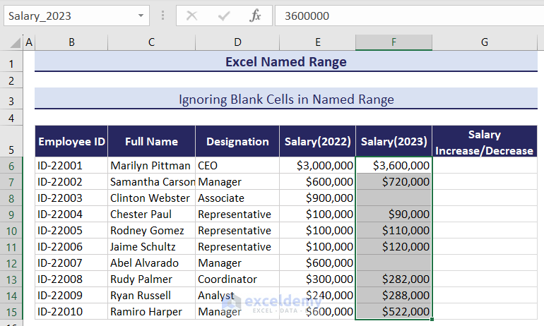
How to Ignore Blank Cells in Excel Named Range

We have a dataset of Salaries from 2022 and 2023 for some employees. Now, we want to calculate the increase or decrease in their salary. But there are some blank cells in the column for 2023 salaries. We need to ignore blank cells in Excel Named range because it can create incorrect results.

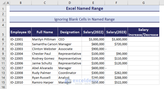
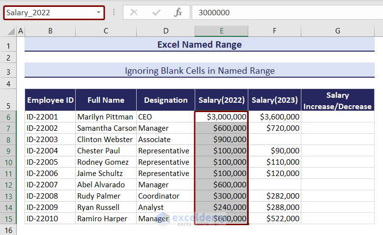
First, we will create a named range for Salary 2022 and Salary 2023 columns.

• Select the cell range of the “Salary (2022)” column.
• Type “Salary_2022” in the Name Box and press Enter.

Click the image to get a better view

Similarly, name the column “Salary (2023)”.

Click the image to get a better view

Now, we will use these two named ranges to calculate salary increases or decreases, ignoring the blank cells.

• For that, insert the following formula in cell G6 and hit Enter.

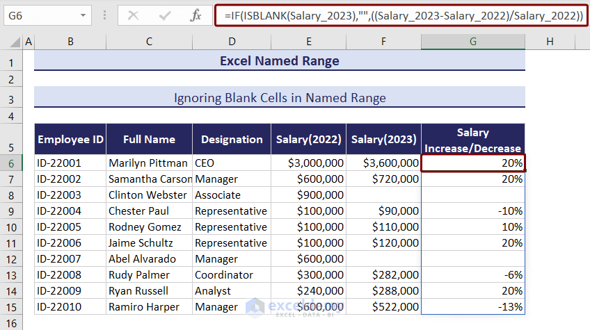
Click the image to get a better view

Here, the ISBLANK function checks if there is any blank in the Salary_2023 named range, and the IF function calculates the salary increase or decrease for the cells that are not blank.

Read More: How to Use Named Range in Excel VLOOKUP Function

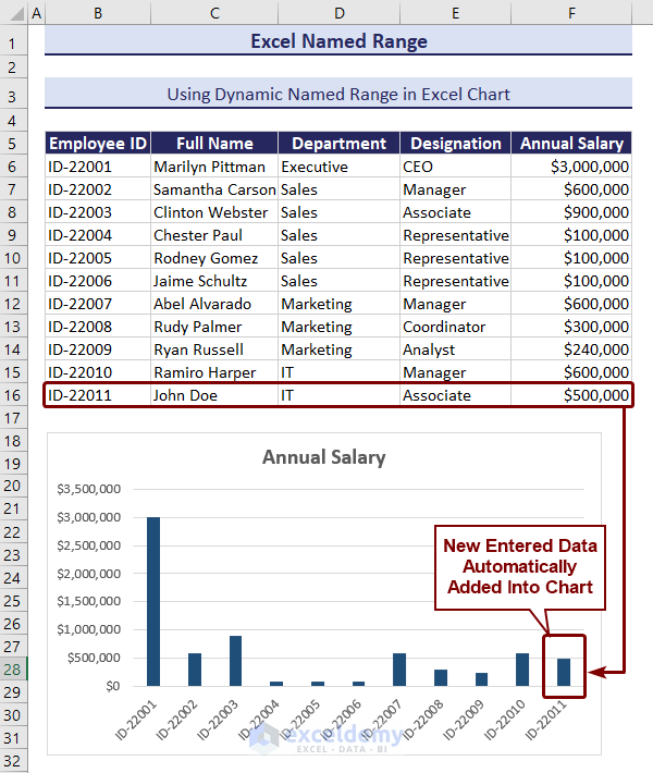
How to Use Dynamic Named Range in Excel Chart

Excel charts visualize data but don’t autofit with new data. To make dynamic charts, use dynamic named ranges. We will create two dynamic named ranges “ID” and “Salary” and then create an Excel chart with them.

• Click on Formulas > Define Name.

• Type “ID” and insert the formula for creating a dynamic named range.

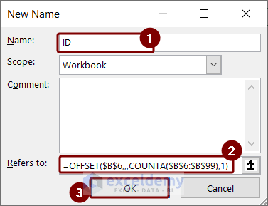
Similarly, we created another dynamic named range, “Salary” using the following formula.

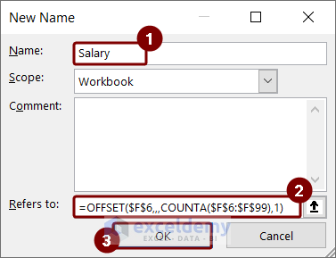
Now that the dynamic named ranges are created, we will insert a chart in the Excel sheet.

• Go to Insert tab.
• From the Charts section, select the 2D Column chart.

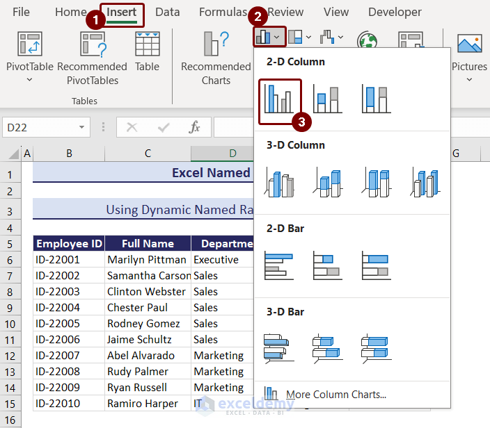
• A blank chart will be inserted in the spreadsheet.
• Right-click on the chart, and from the context menu, click on the Select Data option.

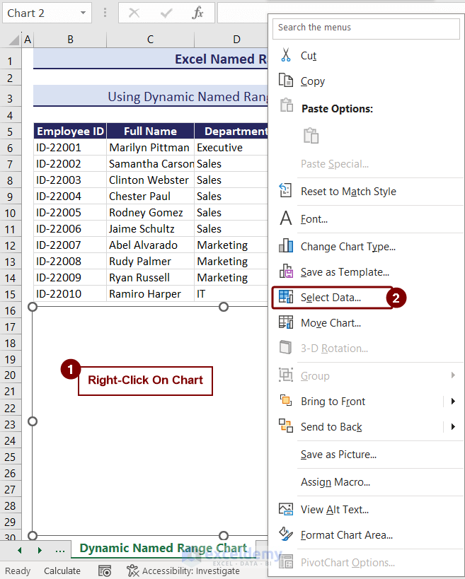
• Now, the Select Data Source named box will appear.
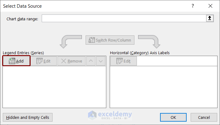
• Click on the Add button under the Legend Entries (Series) option.

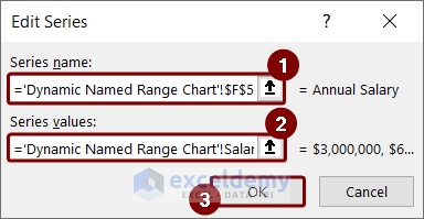
• In the Edit Series box, you will see the Series Name box.
• As a series, we want to enter Salary values, so we entered the cell reference F5 which contains the name Annual_Salary.
• Enter the dynamic named range “Salary” in the Series Values option and press OK.

• Pressing OK will take you back to the Select Data Source box. Now, we will enter employee IDs as Horizontal Axis Labels.
• So, select the Edit option under the Horizontal (Category) Axis Labels option.

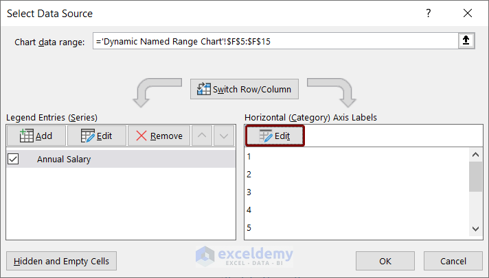
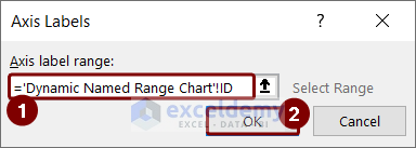
• In the Axis Labels box, enter the dynamic named range, ID, and press OK.

• In the Select Data Source box, you will see the selected dynamic named range is showing.
• Then, press OK.

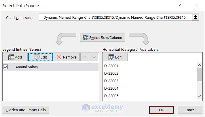
• You will see that the chart shows the values in the dynamic named ranges.

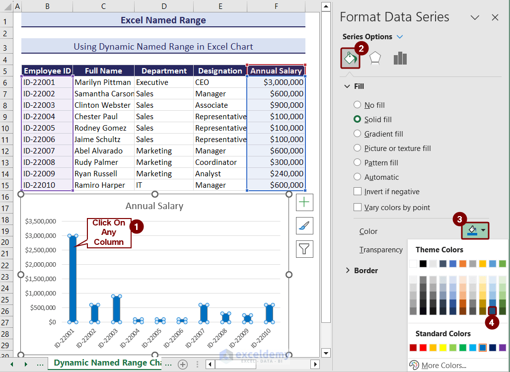
Now, we will change the color of the columns (this is optional).

• For that, double-click on any column, and on the right side of the sheet, you will see the Format Data Series option.
• Select Series Options, and click on the Fill & Line option.
• Then, from the Color option, choose any color of your choice.

Click the image to get a better view

The column’s color has changed, and the chart has become dynamic using the named range. We added a new row of data, and it is visible in the chart.

Tips and Tricks for Excel Named Range

In this part, we will show you some tips and tricks with named ranges.

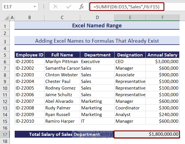
1. Applying Excel Names in Already Existing Formulas

Excel can replace a cell reference with a defined named range if its reference matches.

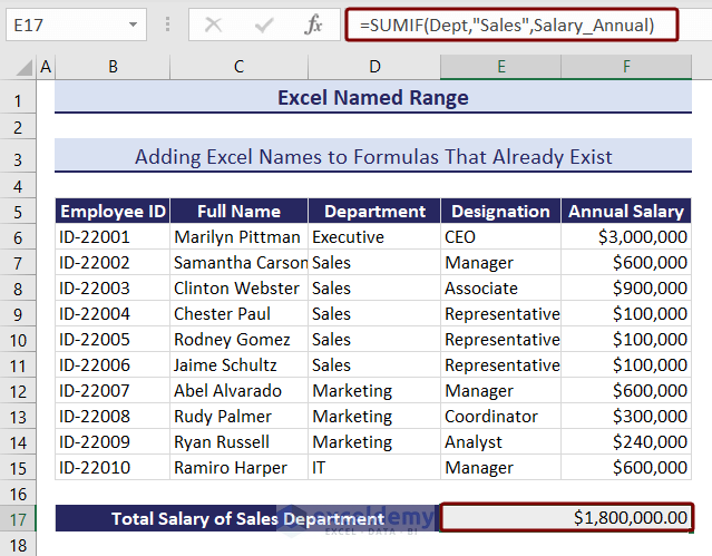
In the image below, we showed a formula for calculating the “Total Salary of Sales Department”.

The formula consists of cell references that we have already named. We can replace these cell references using the Apply Names feature of Excel.

• For that, select cell E17 >> go to the Formulas tab >> click on the Define Name option and select Apply Names.

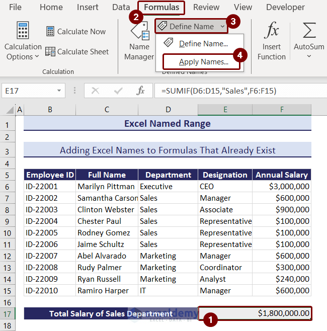
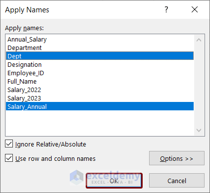
• Apply Names box will appear.
• Dept and Salary_Annual named ranges match with the cell references D6:D15 and F6:F15. So, they got selected automatically.
• Keep the checkboxes Ignore Relative/Absolute and Use row and column names checked and press OK.

In the formula, the cell references were replaced with the named ranges.

Read More: How to Paste Range Names in Excel

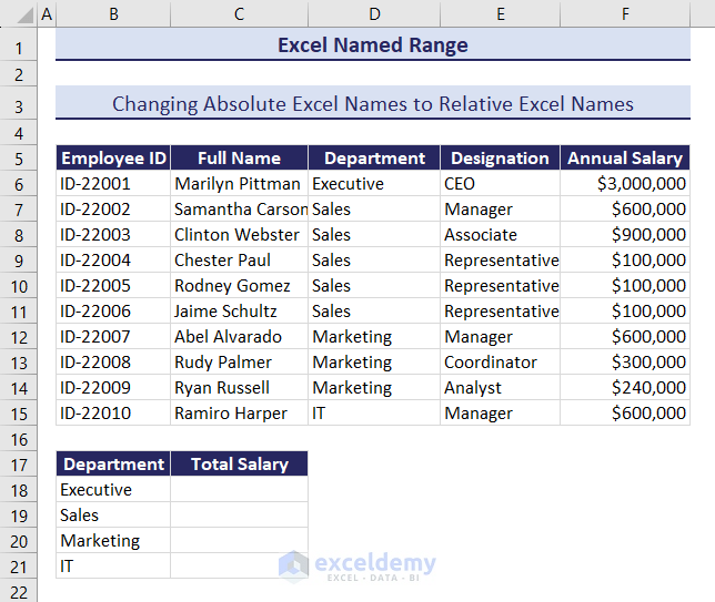
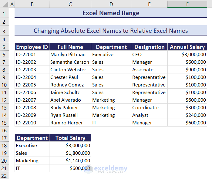
2. Changing Absolute Excel Names to Relative Excel Names

You can define a named range without absolute cell reference, which will change according to the cell where you used the named range. Below, we show you how to calculate the total salaries of each department using relative Excel names.

For that, we have added department names in cell range B18:B21 and added a column where we will apply the formula for calculating total salaries.

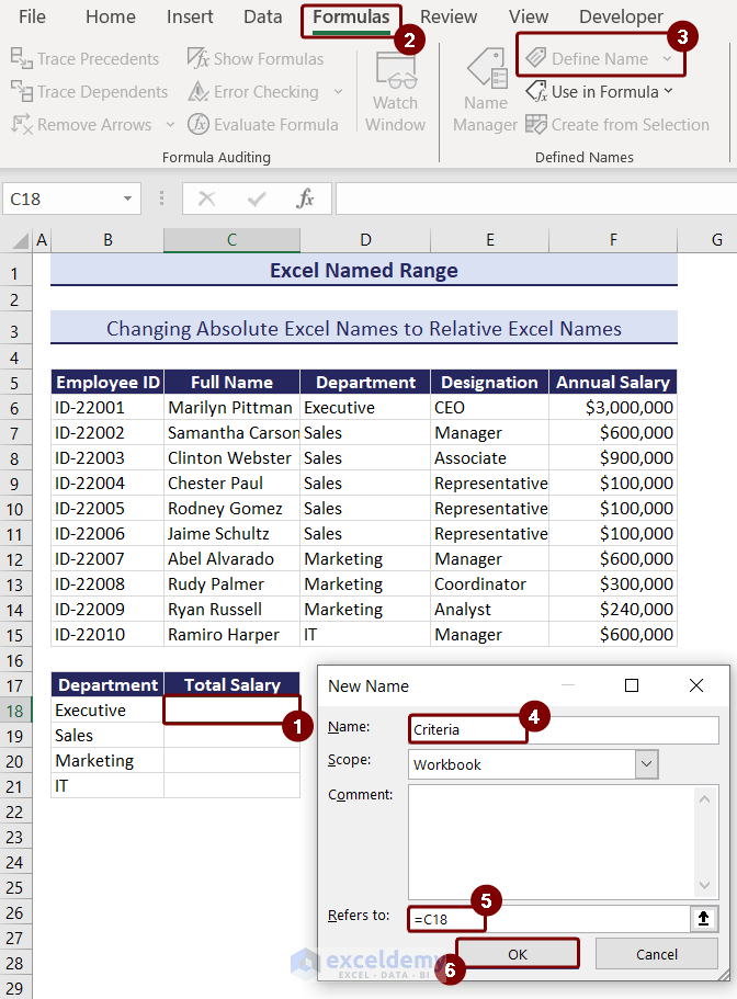
• First, select cell C18 and go to the Formulas tab > Define Name.
• Next, in the New Name box, type Criteria in the name box.
• Type C18 as the relative cell reference in the Refers to box.
• Press OK.

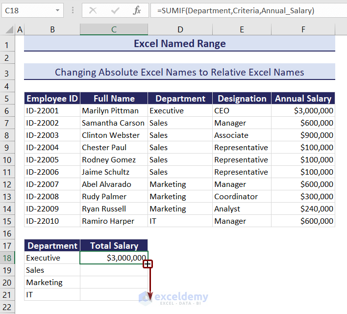
• Now, insert the following formula in cell C18.

Here, in the image you can see that the Department named range defines D6:D15 cell range, Annual_Salary defines F6:F15 cell range. Though we defined cell C18 as Criteria, it is showing B18 as Criteria. This is the beauty of relative Excel names. It changes cell reference with its relative position. 

• Then press Enter to see the total salary of the Executive department.
• Now, drag the Fill Handle to copy down the formula.

• You can see the total salaries of all departments.

Notice that relative cell reference changed at each row according to the position of the formula and thus returned the exact results.

How to Create a Name for a Constant in Excel

We want to calculate the tax amount each employee has to pay from the dataset below.

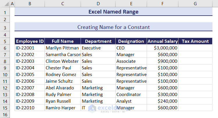
Let us assume the tax rate is 7%, and we will define a named range for this constant value.

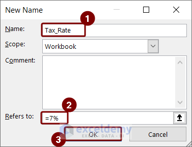
• For that, open the Define Name option from the Formulas tab.
• In the New Name box, type Tax_Rate.
• Enter 7% into the Refers to box and press OK.

• Now select cell G6 and insert the formula containing the named range.

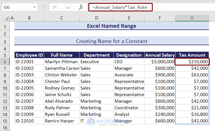
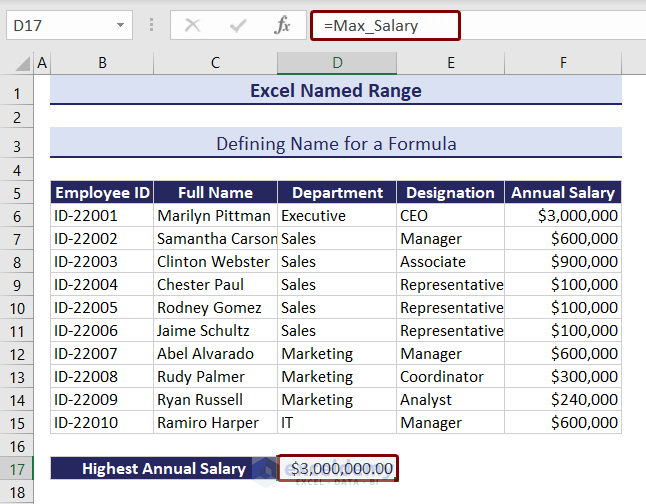
How to Define Name for a Formula in Excel

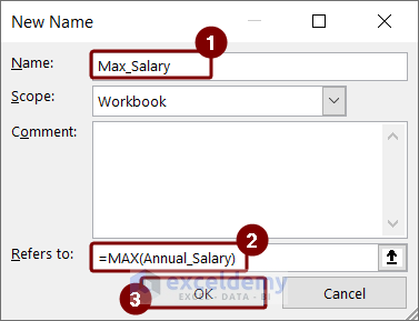
In Excel, you can define a name for a formula to use it multiple times. Let’s define a name for the formula to find the maximum salary of employees.

• First, open the Define Name option from the Formulas tab.
• Type Max_Salary as the Name of the formula.
• In Refers to box, enter the formula below.

• Press OK.

• Next, select cell D17 and type:

• Press Enter to see the result.

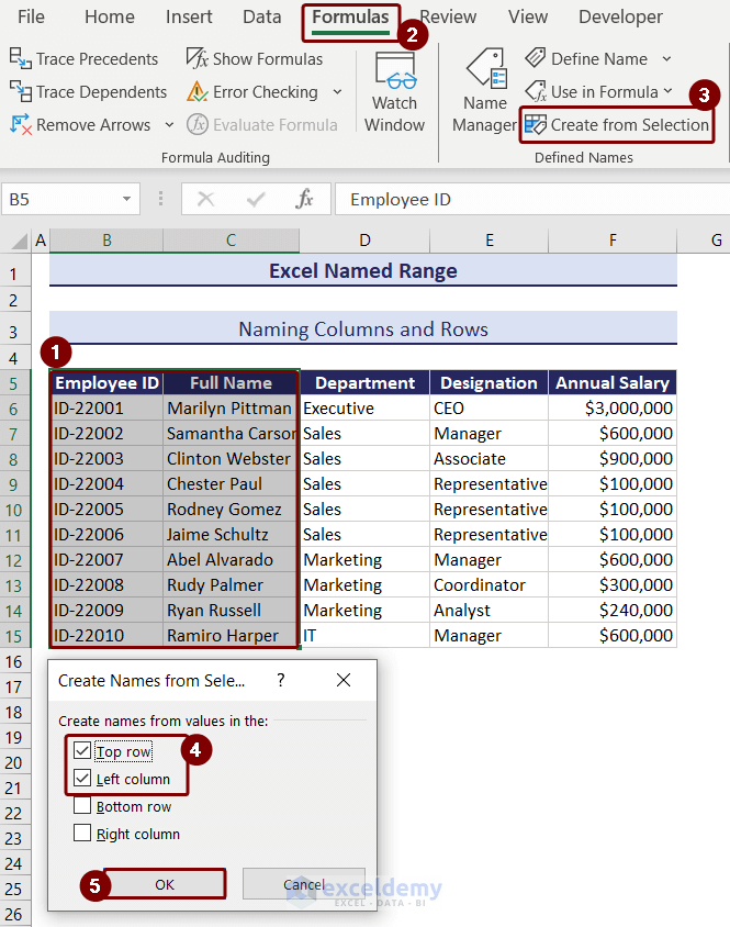
How to Name Columns and Rows in Excel

We can name columns and rows in Excel by using the Create from Selection option.

We will name the Employee ID and Full Name columns and their top rows.

• First, select the cell range B5:C15.
• Then, go to the Formulas tab > Select Create from Selection.
• A box named Create Names from Selection will appear.
• Check the boxes Top row and Left column, as we want to name the selection Employee ID.
• Lastly, press OK.

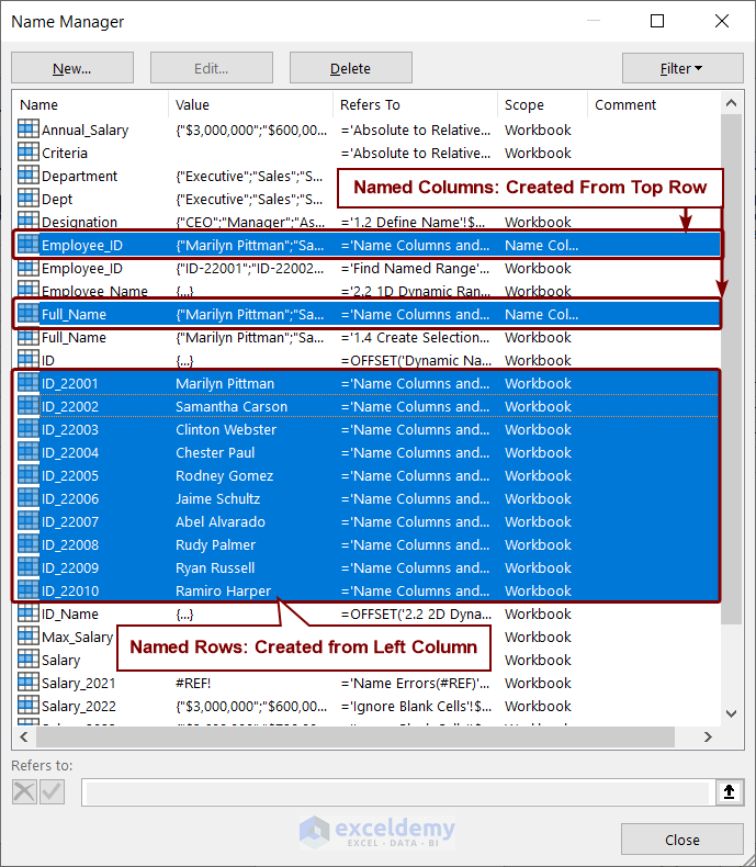
In Name Manager, you can view the created names of columns and rows.

How Do You Use Named Range in Another Sheet?

To use the named range in another sheet, you just have to keep the Scope of the named range as Workbook. This will let you use your named range in any worksheet in that workbook.

In the image, we have a “Designation” named range with a workbook-level scope. We can use this named range in any other worksheet in the workbook.

Read More: How to Name a Group of Cells in Excel

Issues with Named Ranges in Excel

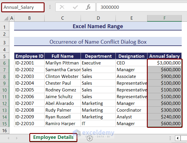
1. Occurrence of Name Conflict Dialog Box

The name conflict dialog box appears when you try to copy one or more sheets into another workbook containing named ranges having a common name.

For example, we have already created Annual_Salary named range in our current workbook, named “Excel Named Range”. We have another workbook named “Employee Details” with the same named range Annual_Salary, shown in the image below.

Now, we will try to copy this sheet to our current workbook, named “Excel Named Range”.

• For that, right-click on the sheet name.
• Choose Move or Copy from the context menu.

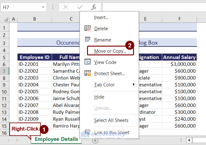
• Next, a box named Move or Copy will show up.
• Click on To book drop-down.
• Choose the workbook name where you want to move or copy the sheet. We selected the “Excel Named Range.xlsx” workbook.

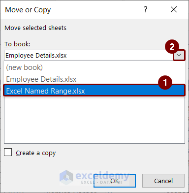
• Now, the sheet names of that book will be available. You can choose where you want to put the copied sheet. We kept it at first.
• Check the Create a copy box and press OK.

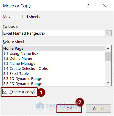
A warning message from Microsoft Excel will pop up stating that the Annual_Salary name already exists with three options. Press:

• Yes: to use that version of the name
• Yes to all: to use that version name for all the name that conflicts at once
• No: to rename the version of the named range you are moving or copying

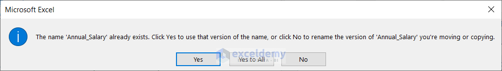
Click the image to get a better view

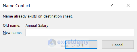
If you press No, then another box named Name Conflict will appear. Here, in the New Name box, you can change the name that conflicts.

Read More: How to Navigate to a Named Range in Excel

2. Occurrence of Name Errors (#REF and #NAME)

While working, deleting some cells or editing might cause errors. Usually, #NAME and #REF errors are the most common to occur. Let us show you why these errors occur and how to solve them.

#NAME Error

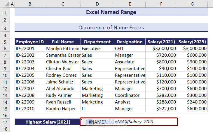
#NAME error occurs when any non-existing name is entered or any name is misspelled.

Like in the image below, we wanted to calculate the highest salary for 2023. But we misspelled the named range. We entered Salary_202 instead of Salary_2023. As a result, Excel is showing a #NAME error.

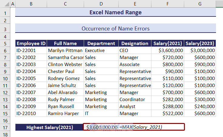
To avoid this error, you just have to enter the correct named range inside the formula. Like in the image below.

#REF Error

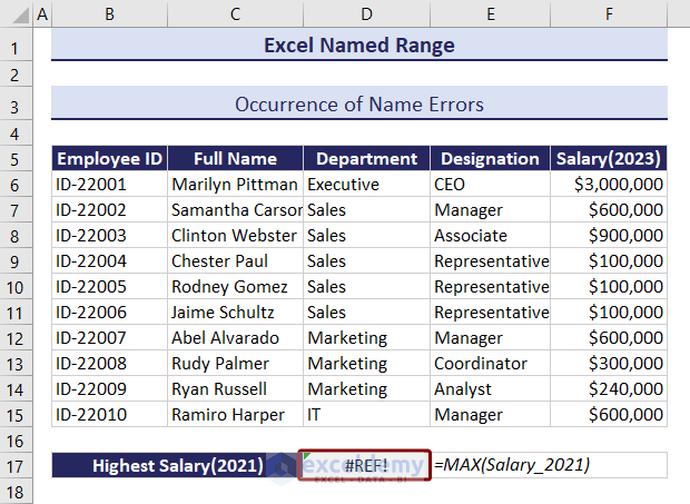
#REF error usually occurs if you delete all cells of a certain named range.

Like in the image below, we calculated the highest salary for 2021 using the named range Salary_2021 which contains cell range F6:F15.

Now, we will delete the F column. Right-click on the F column and select Delete from the context menu.

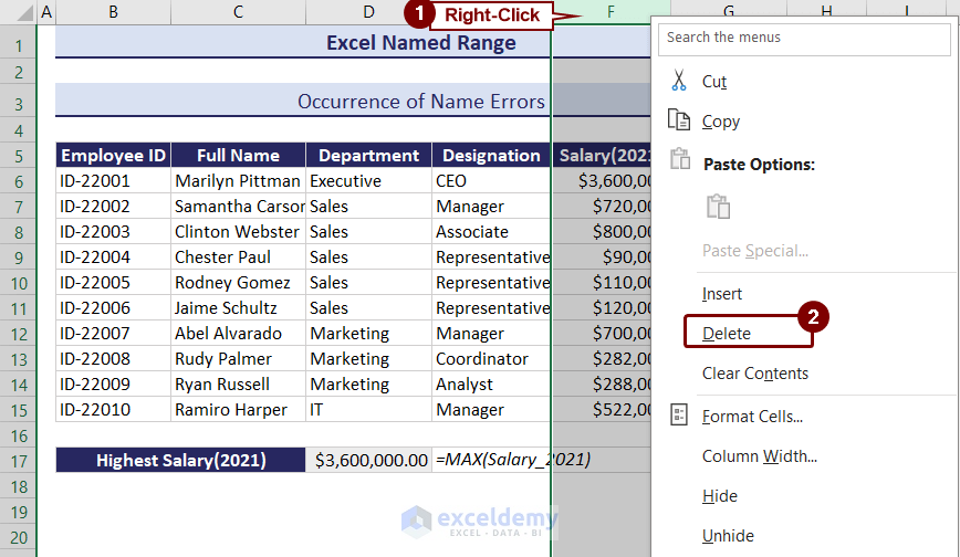
Click the image to get a better view

You can see that a #REF error appeared with the deletion of the column.

To avoid this error, be careful while deleting any data from your dataset. Check if the data you are deleting is part of any named range or not.

Read More: How to Name a Column in Excel 

Download Practice Workbook

In this article, we showed you 4 different ways of creating a named range and 2 ways of creating a dynamic named range. In addition to that, there are demonstrations of how you can find named ranges and keyboard shortcuts to get named ranges creation options. We also discussed editing, filtering, and deleting named ranges using the Name Manager option. Further, we discussed some use cases, tips and tricks, and issues with named ranges. We hope that you have learned all the things about Excel Named Range from this article. If you have any further queries or feedback you can inform us in the comment section.

Excel Named Range: Knowledge Hub

• Excel INDIRECT Function with Named Range
• Excel Reference Named Range in Another Sheet
• How to Use Dynamic Named Range in Excel Chart

<< Go Back to Excel Formulas | Learn Excel