Admittedly, Named Ranges are a quirky and often misunderstood feature of Excel that most people think is pointless. In reality, the issue is that few people are familiar with this unusual but handy feature in Excel. Granted this, in this article, we’ll explore 4 ways how to display Named Range contents in Excel.
The below animated GIF is an overview of this article, which represents how to display Named Range contents in Excel.
In the following sections, you’ll learn what a Named Range is, and each method to display contents of Named Range with the appropriate illustrations.
What Exactly Named Range in Excel Is
In simple terms, a Named Range consists of a range of cells or an array that has a custom (user-defined) name assigned to it. Generally speaking, Name Ranges are an alternative to manually entering a cell range in a function or formula. Moreover, Named Ranges help to make formulas dynamic and easy to understand.
Display Named Range Contents in Excel: 4 ways
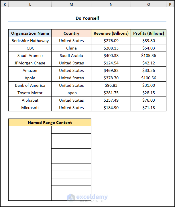
First and foremost, let’s suppose the “Financial Performance of Companies in 2022” dataset containing the “Organization Name”, “Country”, “Revenue”, and “Profits” columns in the B4:E14 cells. Henceforth, let’s see each method in action!
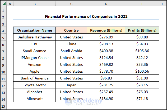
Here, we have used the Microsoft Excel 365 version; you may use any other version at your convenience.
1. Using Paste Names Feature to Display Named Range Contents
In the first place, we’ll begin the simplest and most obvious way, simply put, we’ll use the Paste Names feature to return the range of cells stored within the Named Range.
📌 Steps:
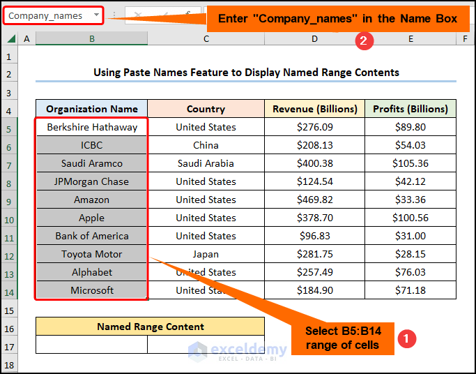
- First, select the B5:B14 cells >> enter a suitable name, here it is “Company_names” in the Name Box >> press the ENTER keys.
Now, this means we can use “Company_names” instead of referencing the B5:B14 cells.
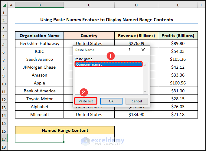
- Second, go to the B17 cell >> move to the Formulas tab >> click the Use in Formula drop-down >> hit the Paste Names button.
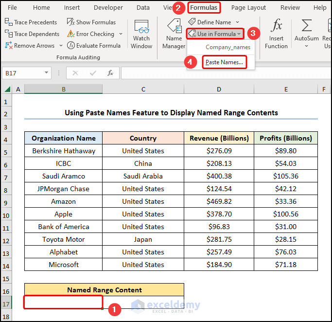
- Next, choose the Named Range, in this case, “Company_names” >> click Paste List.
- Third, select the C17:C26 array >> Left-click on the Formula Bar to enter Editing Mode >> click the CTRL + SHIFT + ENTER keys.
📃 Note: If you’re using a newer version of Excel like Microsoft Excel 365, then pressing only the ENTER key returns the same result.
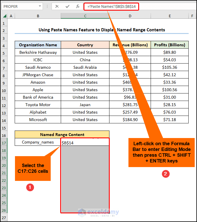
Eventually, the results should look like the image shown below.

Read More: How to Paste Range Names in Excel
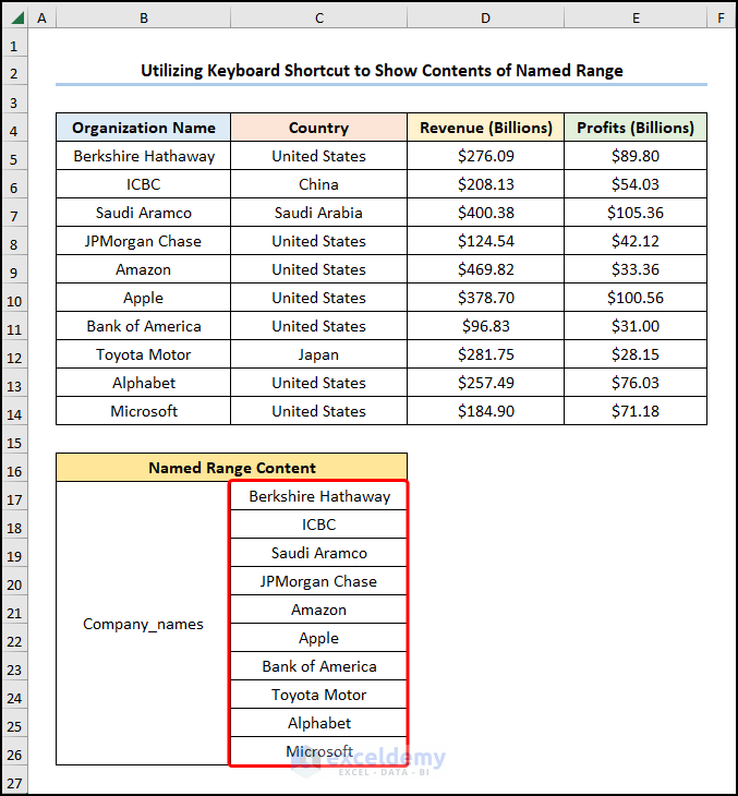
2. Showing Contents of Named Range Utilizing Keyboard Shortcut
Besides, you might be wondering: are there any shortcut keys? Luckily, there are shortcut keys to display the contents of a Named Range and our next method describes just that.
📌 Steps:
- First of all, define the “Company_names” Named Range as shown previously >> highlight the C17:C26 range of cells >> press the F2 key.
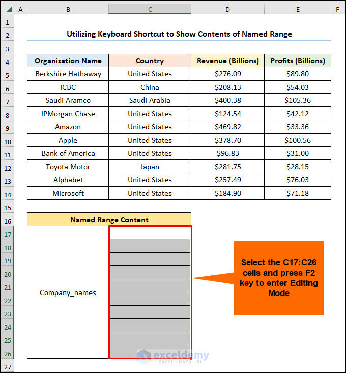
- Then type the name of the Named Range as shown below >> press CTRL + SHIFT + ENTER keys on your keyboard.
=Company_names
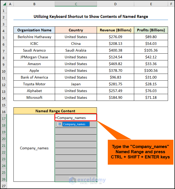
Boom! That is how simple it is to display Named Range contents in Excel.
Lastly, the GIF below recaps the described steps.

Read More: How to Name a Column in Excel
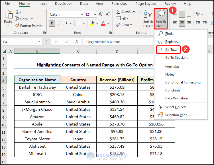
3. Highlighting Contents of Named Range with Go To Option
In addition, we can request Excel to highlight the cells present in the defined Named Range with the help of the Go To option.
📌 Steps:
- To begin with, navigate to Find & Select drop-down >> choose Go To option.
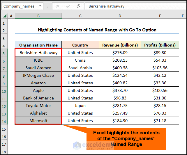
- At this point, click on “Company_names” >> hit OK.
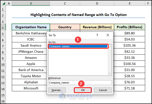
Eventually, the B5:B14 cells stored in the “Company_names” Named Range are highlighted.
Read More: How to Find a Named Range in Excel
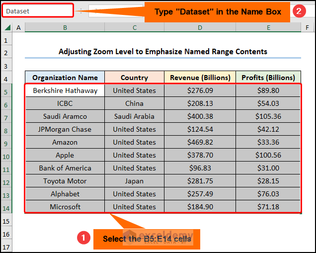
4. Emphasizing Named Range Contents by Adjusting Zoom Level
Last but not least, we can also emphasize the contents of a Named Range by adjusting the Zoom Level of the spreadsheet. In this case, setting the zoom below 40% forces Excel to directly show the Named Ranges.
📌 Steps:
- Initially, choose the B5:E14 cells >> enter the name, “Dataset” in the Name Box >> click on ENTER.
- Afterward, proceed to the View tab >> click the Zoom button.
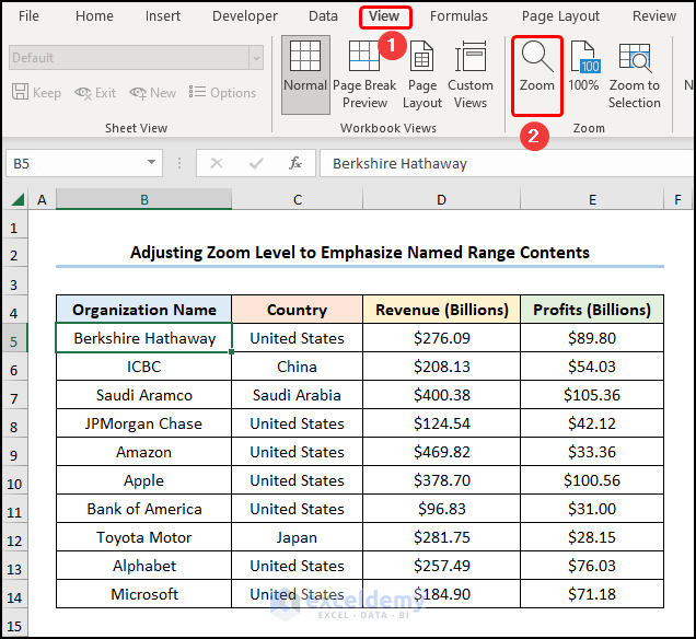
- Not long after, set a custom zoom, for instance, we’ve chosen 39% >> press the OK button.
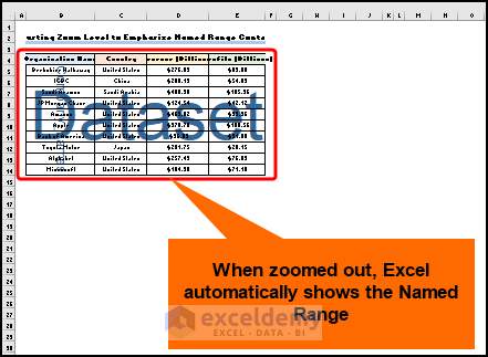
📃 Note: For this method to work, you must set the Zoom Level to below 40%.

Subsequently, the final output should resemble the figure given below.
💡 Things to Remember
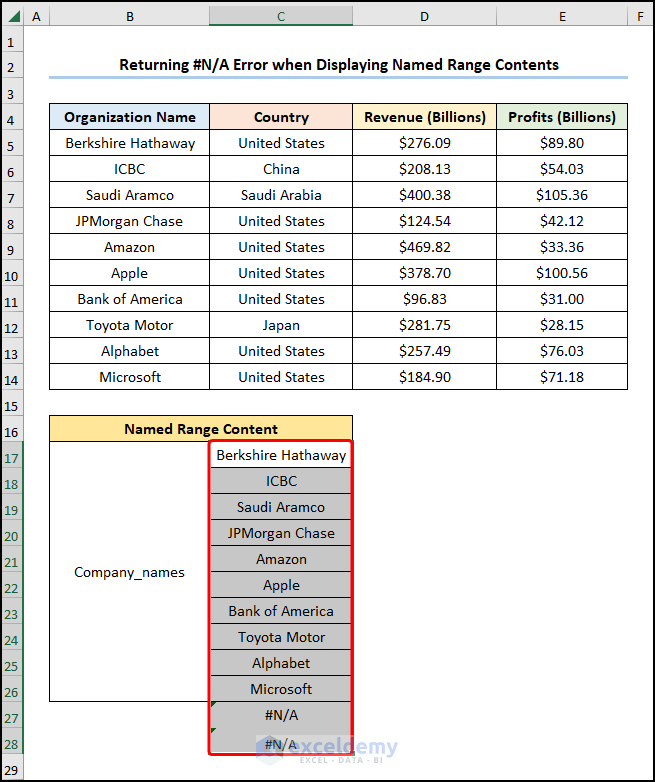
As a note, when displaying the Named Range contents in Excel you may encounter the #N/A error.
- For one thing, if we select a greater number of rows than the rows present in the Named Range then Excel returns the #N/A error.
For example, the “Company_names” Named Range contains 10 rows, however in the picture below, we’ve chosen 12 rows, so the last 2 rows have no available data, hence the #N/A error.
Practice Section
We have provided a Practice section on the right side of each sheet so you can practice yourself. Please make sure to do it by yourself.
Download Practice Workbook
Conclusion
In short, this tutorial explores all the ins and outs of how to display Named Range contents in Excel. Now, we hope all the methods mentioned above will prompt you to apply them to your Excel spreadsheets more effectively. Furthermore, if you have any questions or feedback, please let me know in the comment section.
Related Articles
- How to Navigate to a Named Range in Excel
- How to Name a Group of Cells in Excel
- How to Change Scope of Named Range in Excel
- How to Edit Named Range in Excel
- How to Delete Named Range in Excel
- How to Delete All Named Ranges in Excel
<< Go Back to Named Range | Excel Formulas | Learn Excel
Get FREE Advanced Excel Exercises with Solutions!
