How to Name a Group of Cells in Excel (3 Easy Methods)

Although naming ranges of cells is one of the most useful features in Excel, making formulas more readable, easy to understand, and maintainable, it is not commonly used. In this article, we will show you how to name a group of cells in Excel through 3 easy methods (with one bonus) and use these named cells with an example at the end.

how to name a group of cells in excel

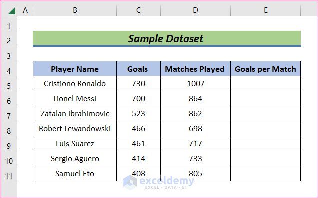
We’ll use the dataset above, containing 7 soccer players with their career goals and the number of matches played, and name two groups of cells in this dataset by means of 3 easy methods. Then we’ll use those named cells in a formula to calculate the number of matches required for each player to score a goal.

Note: Naming cells should follow the naming convention defined by Microsoft Excel.

Method 1 – Using the Name Box

We can name a group of cells in Excel by typing a name in the Name Box.

Steps:

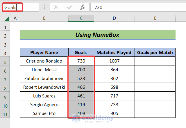
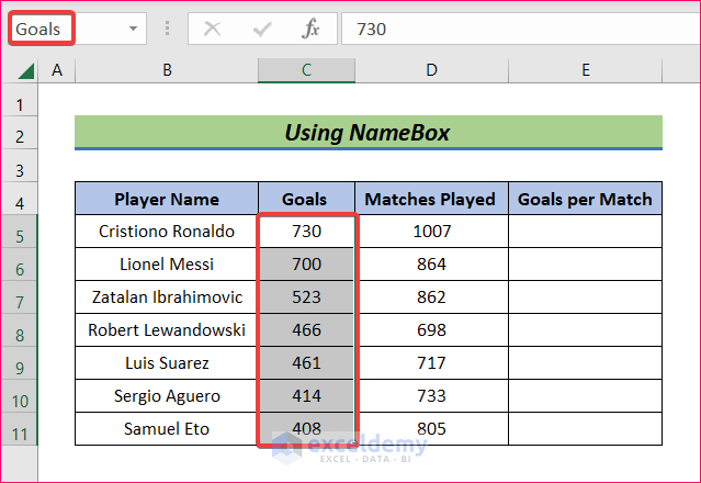
Select the range of cells C5:C11 by dragging the mouse.

In the NameBox (top-left corner of the worksheet), only the column reference C5 is displayed.

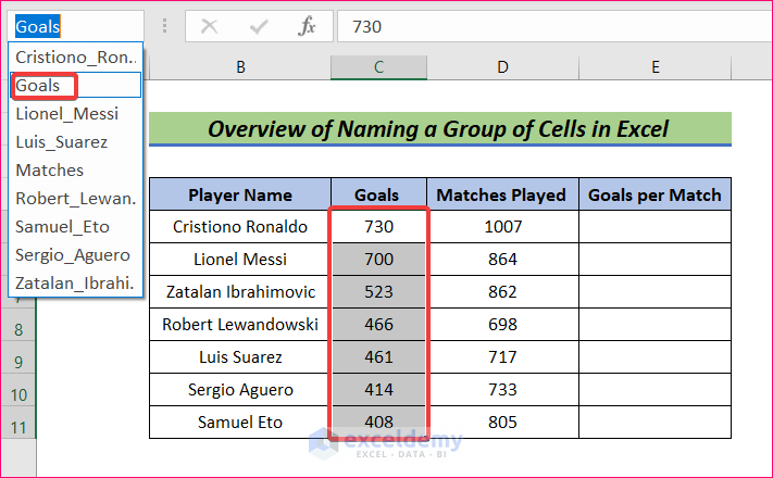
Enter a name in NameBox (Goals in this example) and press Enter.

If we select the cell group again, the NameBox shows the given name (Goals).

Read More: How to Name a Column in Excel

Method 2 – Using the Define Name Option

We can also use the Define Name option in the Formula tab.

Steps:

Select the Formulas tab and click the Defined Names option.

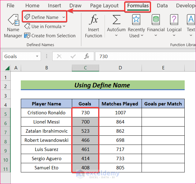
A dialog box in which to insert a name for the range opens.

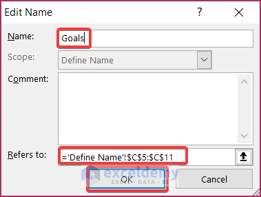
Enter Goals in the input box and click OK to finish the process.

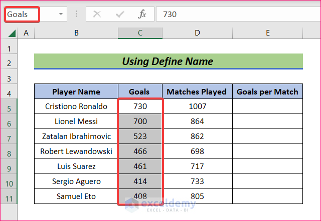
The name of the group of cells now appears in the NameBox.

Read More: How to Edit Named Range in Excel

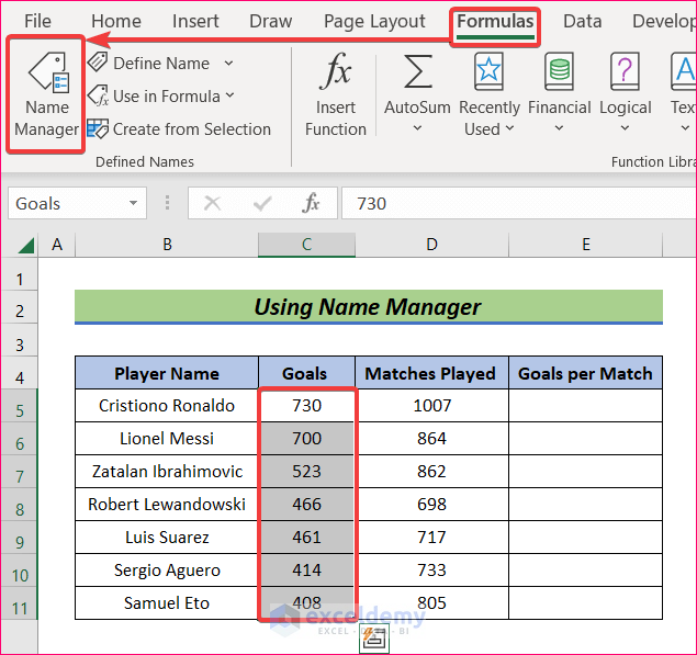
Method 3 – Using the Name Manager

Another way to name a group of cells is to use the Name Manager in the Formulas tab.

Steps:

Select the range of cells C5:C11.
Select the Formulas tab and then the Name Manager option.

In the Name Manager window, click the New button.

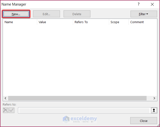
A new window pops up.

Enter our desired name (Goals) and click OK to save.

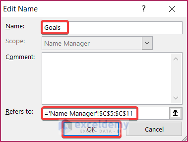
Our cell range is named.

Let’s Check:

The above 3 methods enabled us to name the range C5:C11 as Goals.

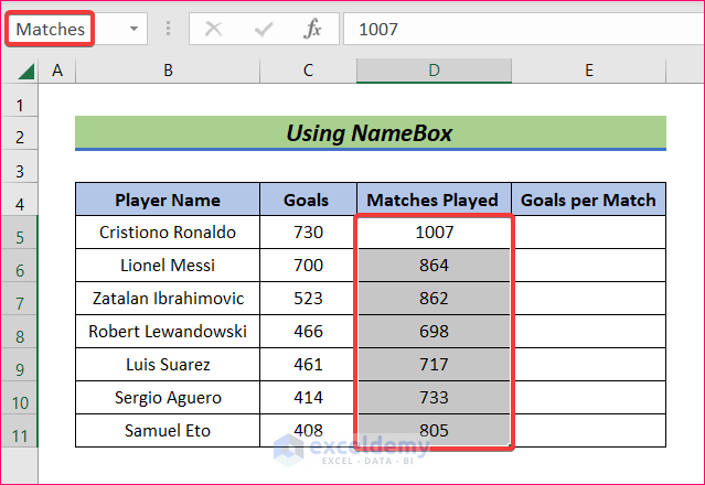
Name D5:D11 as Matches using any of the three methods.

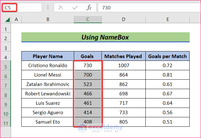
Now, let’s divide the Goals column by the Matches column to get Goals per Match for each player.

In cell E5, enter the following formula:

=Goals/Matches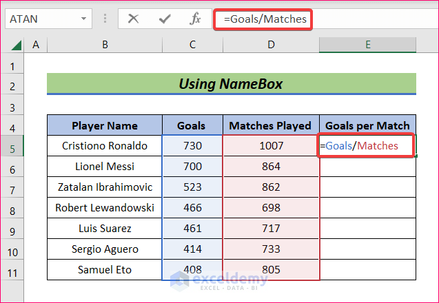

Press Enter.
Apply the same formula in cells E6:E11 by dragging the Fill Handle down.

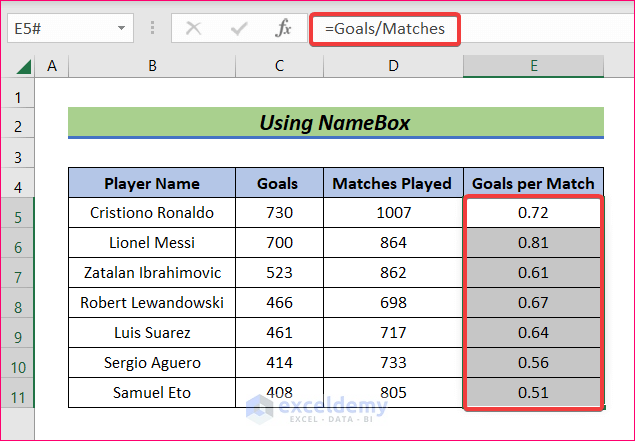
The names ranges greatly simplify our formula syntax.

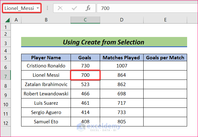
Using Create From Selection Option to Name Grouped Cells

If your data is organized in a tabular form, this bonus method will enable you to give a name to each cell of a column corresponding to another column’s cells.

Steps:

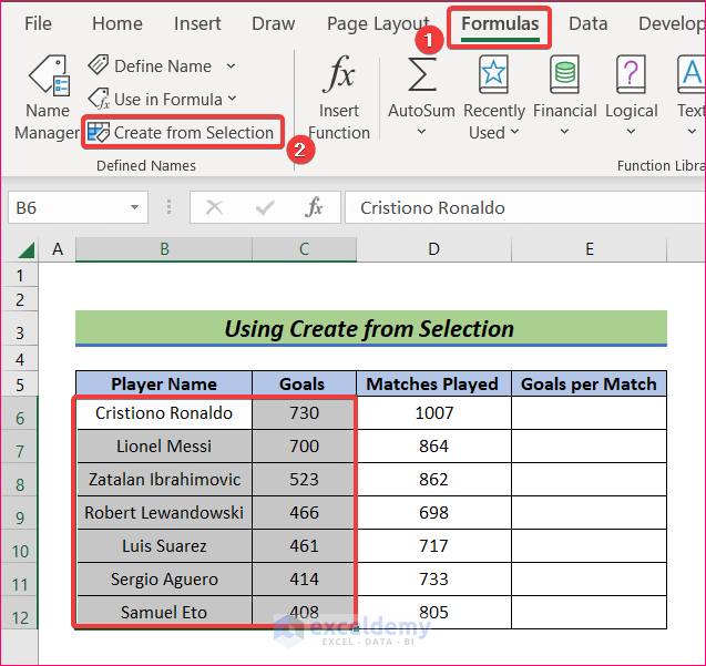
Select the two columns B5:B11 and C5:C11.
From the Formulas tab, select the Create from Selection option.

Select Left Column from the Create Names from Selection tab that opens.
Click OK.

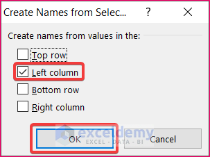
Now if we select any of the cells in the Goals column, the NameBox shows the corresponding name of the player from the Player Name column. The Player column is on the left of the Goals column, which is why we selected the left column option in the previous step.