Step 1 – Preparing the Dataset for a Dynamic Named Range in Excel
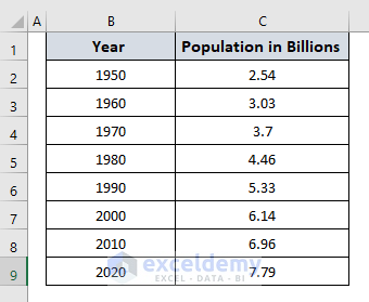
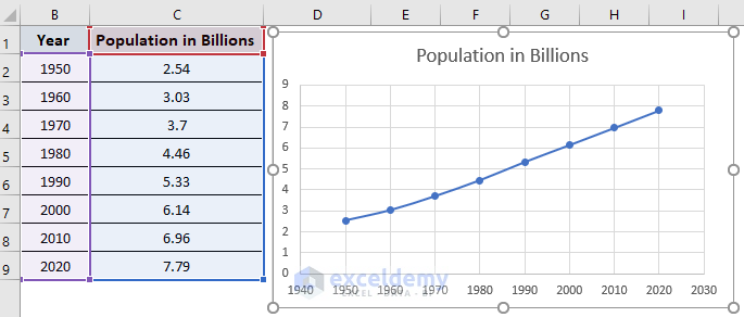
We’re going to use the following dataset that illustrates the growth of the world population from 1950 to 2020. We want to make the dataset dynamic with the use of named ranges. When we add a new row of data, the range will expand accordingly.
Step 2 – Creating a Dynamic Named Range to Use in a Chart in Excel
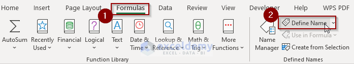
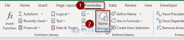
- Go to the Formulas tab in the Ribbon.
- Click the Define Name option.
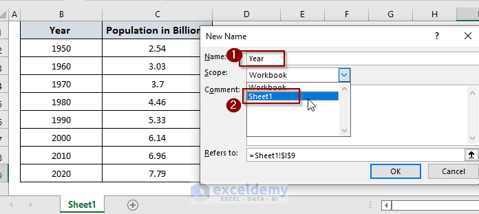
- In the New Name window, type Year (same as the header name, for convenience) in the Name input box.
- In the Scope dropdown list, select the Sheet1 option as our dataset is in the Sheet1 of the workbook.
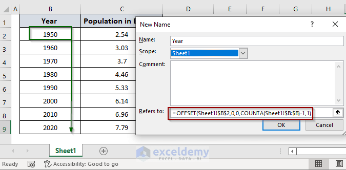
- In the input box named Refers to, put the following formula:
=OFFSET(Sheet1!$B$2,0,0,COUNTA(Sheet1!$B:$B)-1,1)- Hit OK to save the settings.
- Follow the same procedure to make the Population in Billions column a dynamic named range. Use the following formula:
=OFFSET(Sheet1!$C$2,0,0,COUNTA(Sheet1!$C:$C)-1,1)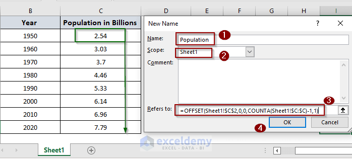
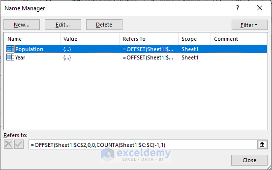
- To check the named ranges, click on the Name Manager button from the Formulas tab.
- In the Name Manager window, there are two name ranges: Year and Population.
Formula Breakdown
=OFFSET(Sheet1!$B$2,0,0,COUNTA(Sheet1!$B:$B)-1,1)The syntax of the OFFSET function is-
=OFFSET(reference, rows, cols, [height], [width])
The function returns a reference to a range, where
reference– the starting point, in our formula, Sheet1!$B$2- is the first cell value in the Year column.
rows- a row offset, set it to 0 in our formula.
cols- a column offset, set it to 0 in our formula.
[height]- the height of the returned range. We used the COUNTA function to count all the no empty cells in column B. Here we subtracted 1, as the column has a header. Leave it if the column has no header.
[width]- the width of the returned range. Always set it to 1.
Read More: Excel INDIRECT Function with Named Range
Step 3 – Using the Dynamic Named Range in an Excel Chart
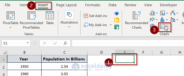
- Select an empty cell in the worksheet at a suitable place.
- Go to the Insert tab in the Excel Ribbon.
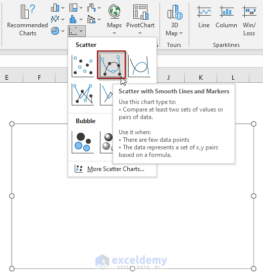
- Click on the Scatter Chart.
- Choose a chart.
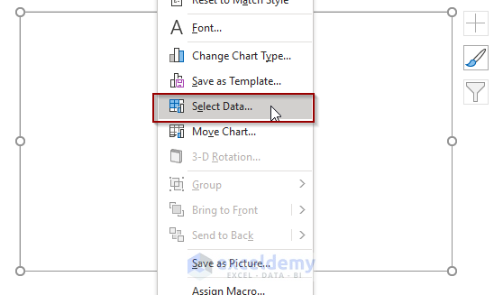
- Right-click on the chart.
- Choose Select Data.
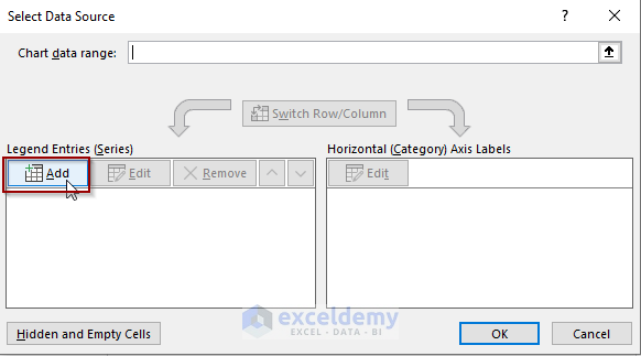
- In the Select Data Source window, click on the Add button.
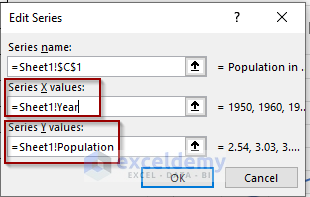
- Click on the header of the column “Population in Billions” to set the series name.
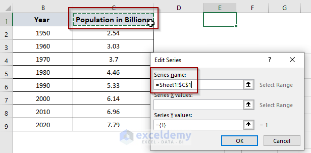
- Put “=Sheet1!Year” in the Series X values input box to display the year values in the x ordinate. The dynamic named range Year belongs to Sheet1, as we defined earlier.
- Put “=Sheet1!Population” in the Series Y values input box.
- Hit Enter.
- Click on the OK button.
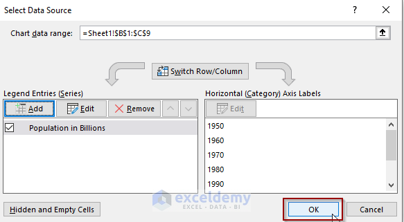
- We’ve got the scatter plot showing the Year–Population relation.
Read More: Excel Reference Named Range in Another Sheet
Step 4 – Checking the Dynamic Named Range in Excel Chart
- Put two more rows in the dataset.
- Enter the predicted population for the years 2030 and 2040 in the dataset.
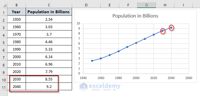
- The chart adjusted with two new entries automatically.
Download the Practice Workbook
Related Articles
<< Go Back to Named Range | Excel Formulas | Learn Excel
Get FREE Advanced Excel Exercises with Solutions!

I use both the OFFSET-version above, the new dynamic arrays, like $A$1#, and named ranges as chart series data references to have the charts dynamic. However, it seems that Excel replaces them with fixed addresses when I copy a sheet to a new workbook. (I have worksheet scope on the named ranges). Would you have any idea why and maybe a workaround for this problem?
Hello JOHAN,
First, thanks for your query. Actually, dynamic named ranges created with OFFSET, and COUNTA functions don’t work when copied to another workbook. You can use a workaround instead. Follow the steps below.
• At first, open the Name Manager.
• Then, click on any name and tap on the Edit button.
Instantly, it will open the Edit Name dialog box.
• Here, change the previous formula in the Refers to box and give this new one.
=INDEX(Sheet1!$B$2:$C$23,0,MATCH(Sheet1!$C$2,Sheet1!$B$2:$C$2,0))• As usual, click OK.
• Similarly, do the same for the second name also. The formula for this is similar also.
=INDEX(Sheet1!$B$2:$C$22,0,MATCH(Sheet1!$B$2,Sheet1!$B$2:$C$2,0))Now, watch the GIF. It’s working in the new workbook.
And the chart is still dynamic. It’s changing while you are inputting new values.
That’s all from me on this topic. Hope you find this helpful. Follow our website ExcelDemy to explore more about Excel. Happy Excelling.
Regards
SHAHRIAR ABRAR RAFID
Excel & VBA Content Developer
Team ExcelDemy
This does not seem to work in a existing chart (Mac OS, Excel v16.16).
I have defined names correctly,
Date=OFFSET(Combined!$A$2,0,0,COUNTA(Combined1!$A:$A)-1,1)
Value=OFFSET(Combined!$B$2,0,0,COUNTA(Combined!$B:$B)-1,1)
but replacing =SERIES(“Combined”,Combined!$A$2:$A$56,Combined!$B$2:$B$56,1) in the chart with
=SERIES(“Combined”,Combined!Date,Combined!Value,1) results in an error
“Excel found a problem with one or more formula references in this worksheet.
Check that the cell references, range names, defined names, and links to other workbooks in your formulas are all correct.”
Hello Don,
It seems you’re facing issues with dynamic named ranges on Mac OS Excel v16.16. Our article is written based on based on Windows OS Excel 365.
Here are some steps you may try to troubleshoot the problem.
Date =OFFSET(Combined!$A$2, 0, 0, COUNTA(Combined!$A:$A)-1, 1)
Value =OFFSET(Combined!$B$2, 0, 0, COUNTA(Combined!$B:$B)-1, 1)
When replacing the series formula in your chart, ensure it looks like this.
=SERIES(“Combined”, Combined!Date, Combined!Value, 1)
If automatic updates are causing errors, manually update the data ranges:
1. Right-click on the chart and select Select Data.
2. Edit the series and input the named ranges manually.
Ensure that your Excel on Mac OS is up to date. Sometimes, these issues are resolved with software updates. There might be compatibility issues between Windows Excel 365 and Mac OS Excel v16.16. Dynamic named ranges sometimes behave differently across platforms.
Regards
ExcelDemy
Found part of the problem, apparently Excel 2016 on Mac only allows Workbook named ranges, so it replaced the worksheet reference (Combined!…) with the workbook name (‘Workbook Name.xlsx’!…). However, still refused to actually apply the result to EXISTING charts, only works with NEW charts.
Hello Don,
Thanks for your feedback! This article is written based on the Windows version of MS Office 365, where dynamic named ranges works across charts.
It seems Excel 2016 on Mac behaves differently, allowing only workbook-level named ranges and replacing worksheet references with the workbook name. Unfortunately, for existing charts, this dynamic range may not apply correctly, and creating new charts might be the only solution on Mac.
We appreciate your insight, and we’ll consider these differences in future content!
Regards
ExcelDemy