This will be the final output:
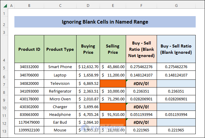
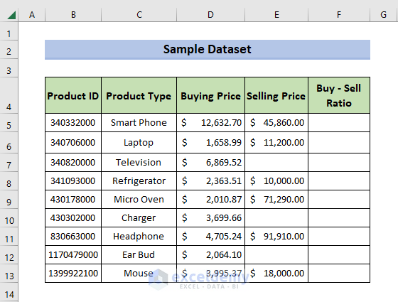
The dataset showcases “Buying Price” and “Selling Price”. There are blank cells in “Selling Price”.
To find the “Buy – Sell Ratio” values, ignoring the errors:
Method 1 – Use of IF Function to Ignore Blank Cells in Named Range
Steps:
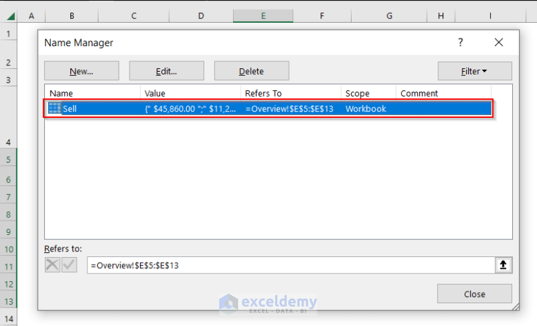
- Create a Named Range: select all cells in “Selling Price” and go to Formulas > Name Manager > New.
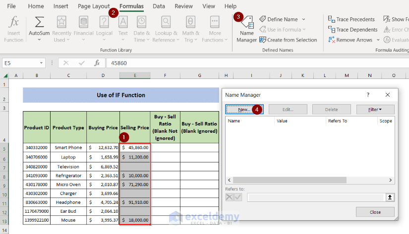
- Select New.
- Enter “Sell” in the Name box and click OK.
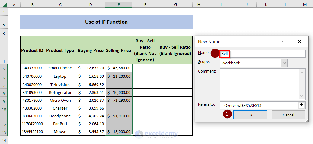
- The Named Range “Sell” is created. A pop-up window will show the details of the Named Range.
- Select Close.
- Create the Named Range “Buy”.
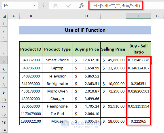
- Enter the following formula in F5.
=IF(Sell="","",Buy/Sell)- Press Enter.
This is the output:
Formula Breakdown:
- =IF(Sell=””,””,Buy/Sell): checks whether the value in the Sell named range is blank. If the value is blank, the IF function ignores that cell and calculates Buy/Sell. It returns the values in Buy – Sell Ratio.
Read More: Excel INDIRECT Function with Named Range
Method 2 – Using the ISBLANK Function
Steps:
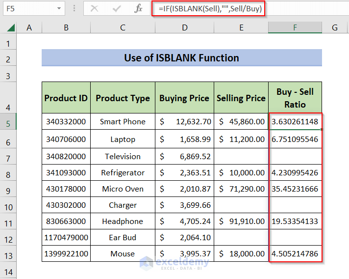
- Enter the following formula in F5.
=IF(ISBLANK(Sell),"",Sell/Buy)- Press Enter.
- This is the output:
Formula Breakdown:
- ISBLANK(Sell): ISBLANK checks whether the value in the Sell named range is blank. If the value is blank, the IF function ignores that cell and calculates Buy/Sell. It returns the values in the Buy – Sell Ratio.
Read More: How to Use Named Range in Excel VLOOKUP Function
Method 3 – Using the ISNUMBER Function to Ignore Blank Cells in a Named Range
Steps:
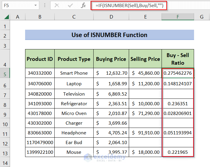
- Enter the following formula in F5.
=IF(ISNUMBER(Sell),Buy/Sell,"")- Press Enter.
- This is the output:
Formula Breakdown:
- ISNUMBER(Sell): ISNUMBER checks whether the value in the Sell named range is a numeric value. If the value is numeric, the ISNUMBER function calculates Buy/Sell or ignores that cell. The IF function returns the values in Buy – Sell Ratio.
Method 4 – Extract Cells Data from a Named Range Ignoring Blank Cells
Steps:
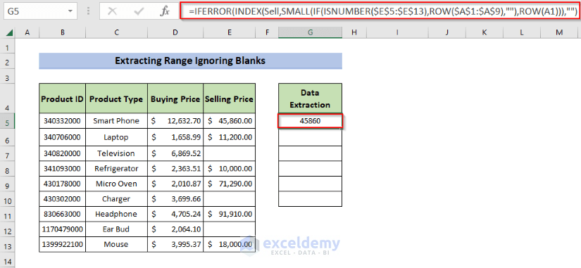
- Enter the following formula in G5.
=IFERROR(INDEX(Sell,SMALL(IF(ISNUMBER($E$5:$E$13),ROW($A$1:$A$9),""),ROW(A1))),"")- Press Enter.
- This is the output:
Formula Breakdown:
- ISNUMBER($E$5:$E$13): returns TRUE for numbers, FALSE otherwise. The output will be TRUE for the non blank cells and FALSE for the blank cells.
Output: {TRUE; TRUE; FALSE; TRUE; TRUE; FALSE; TRUE; FALSE; TRUE}
- ROW($A$1:$A$9): returns the row numbers.
Output: {1; 2; 3; 4; 5; 6; 7; 8; 9}
- IF(ISNUMBER($E$5:$E$13),ROW($A$1:$A$9),””) is simplified as
IF({TRUE; TRUE; FALSE; TRUE; TRUE; FALSE; TRUE; FALSE; TRUE},{1; 2; 3; 4; 5; 6; 7; 8; 9},””). returns the row numbers for TRUE and blank otherwise.
Output: {1;2; “” ; 4; 5; “”; 7; “”; 9}
- ROW(A1): returns the row number of the cell in the argument.
Output: 1
- SMALL(IF(ISNUMBER($E$5:$E$13),ROW($A$1:$A$9),””),ROW(A1))) is simplified as
SMALL({1;2; “” ; 4; 5; “”; 7; “”; 9},1) and returns the 1st smallest value in the range
Output: 1
- INDEX(Sell,SMALL(IF(ISNUMBER($E$5:$E$13),ROW($A$1:$A$9),””),ROW(A1))):
INDEX(Sell,1) returns the 1st non blank value in the range.
Output: 45860
- IFERROR(INDEX(Sell,SMALL(IF(ISNUMBER($E$5:$E$13),ROW($A$1:$A$9),””),ROW(A1))),””) now resembles
IFERROR(45860, “”) returns 45860 as the final output, blank if any error happens
Output: 45860
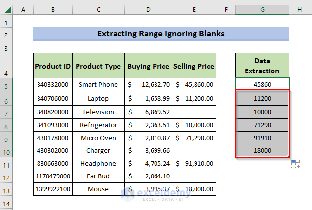
- Drag the AutoFill icon to the end of the list.
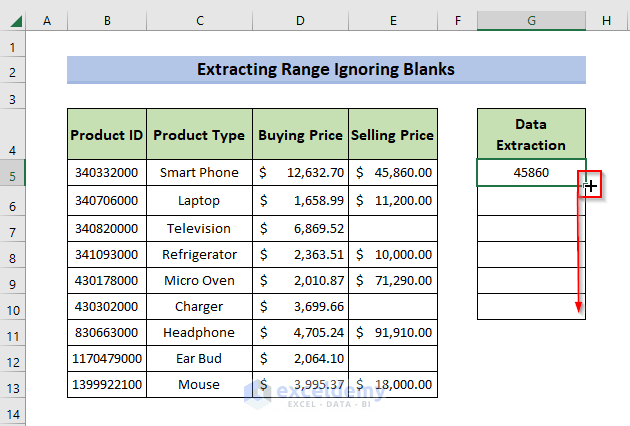 The final output contains all non blank cells in the Named Range Sell:
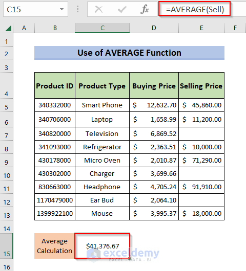
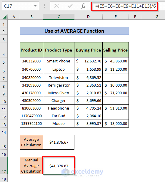
Method 5 –Ignore Blank Cells in a Named Range Using the AVERAGE Function
Calculate the average of the Named Range Sell:
Steps:
- Enter the following formula in C15.
=AVERAGE(Sell)- Press Enter.
This is the output:
- To verify the output of the AVERAGE function: enter the following formula in C17.
=(E5+E6+E8+E9+E11+E13)/6 - Press Enter.
- This is the output:
Download Practice Workbook
Download the workbook.
Related Articles
- How to Create Dynamic Named Range in Excel
- How to Use Dynamic Named Range in an Excel Chart
- Excel Reference Named Range in Another Sheet
<< Go Back to Named Range | Excel Formulas | Learn Excel
Get FREE Advanced Excel Exercises with Solutions!
