How to Name a Column in Excel (3 Easy and Effective Ways)

Method 1 – Using Table Title to Name a Column in Excel

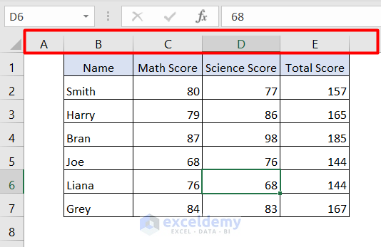
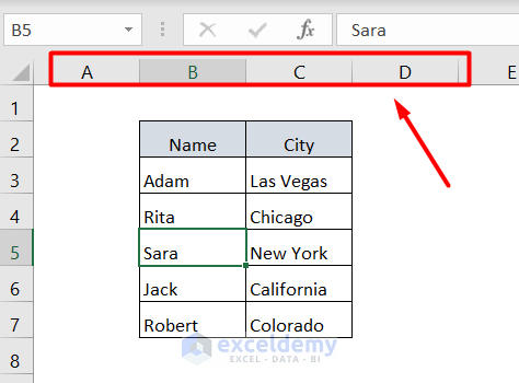
In the following table, we can see that the columns are represented by the English letters A, B, C, and so on. We want to remove the column letters.

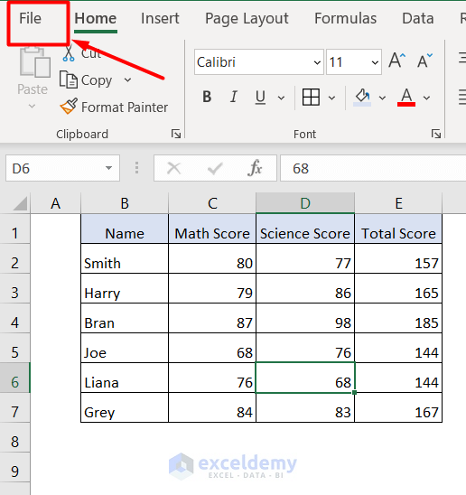
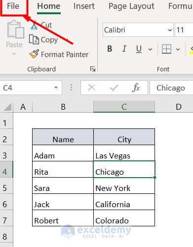
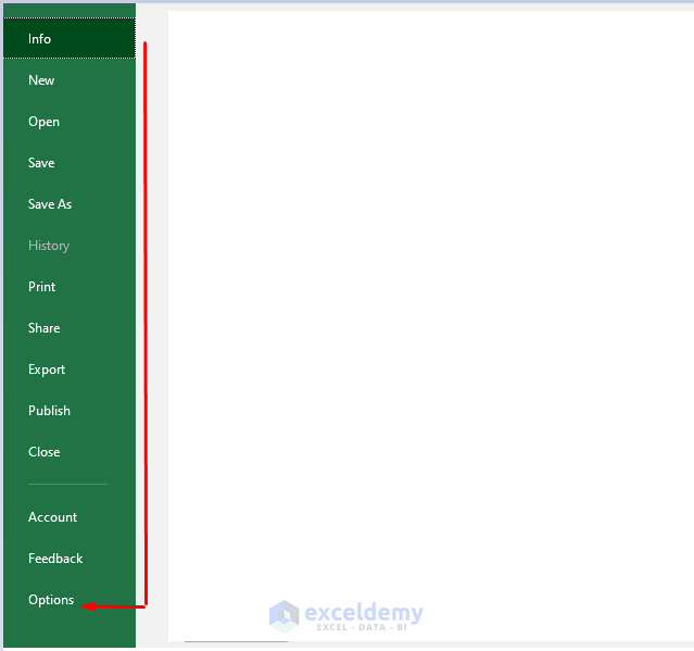
• Select the File option on the top left.

• Select Options.

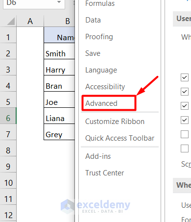
• Click on the Advanced option.

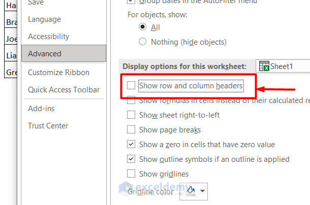
• Scroll down to Display options for this worksheet.

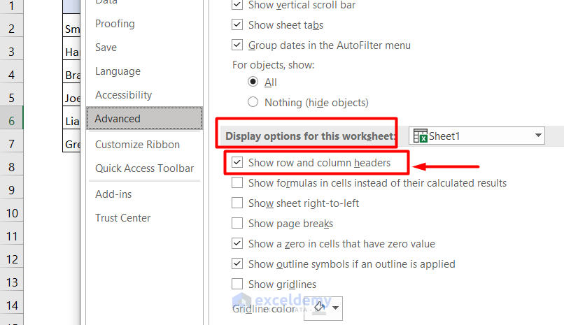
• Unmark the Show row and column headers box and click OK.

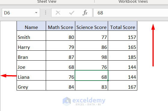
• The column and row headers are gone.

Read More: How to Name a Group of Cells in Excel

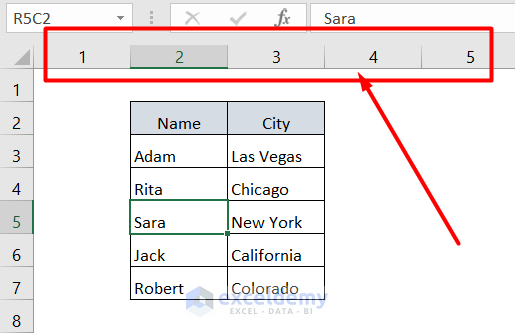
Method 2 – Naming a Column in Excel with a Number

We want to identify the columns by number instead of letter.

• Go to File.

• Select Options.

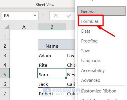
• Select Formulas.

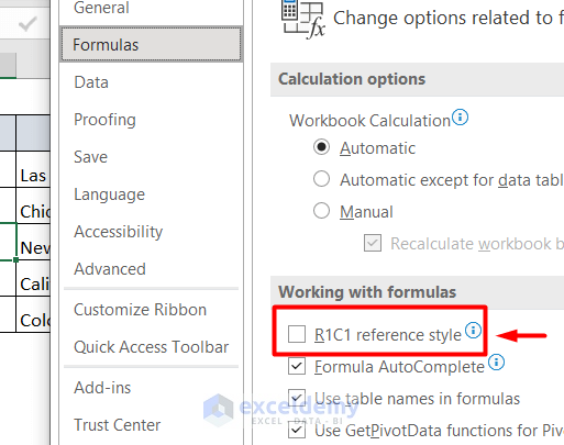
• You will see an unmarked R1C1 reference style box.

• Check R1C1 reference style and click OK.

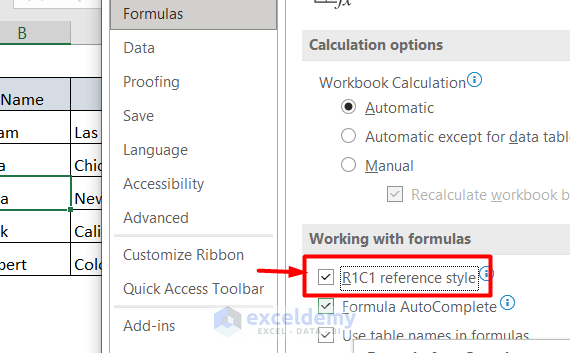
• The column letters are replaced with numbers.

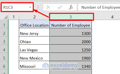
Method 3 – Renaming a Column Name in Excel

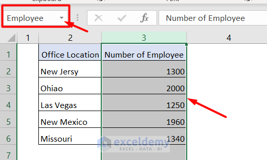
In the following picture, when we select Column 3, it shows the Column Name as R1C3. We want to rename this R1C3.

• Select column 3 and click into the textbox with R1C3. 

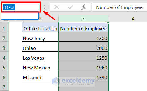
• Delete the R1C3.

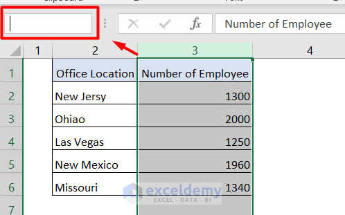
• Type a new column name. We typed Employee.
• Hit Enter.

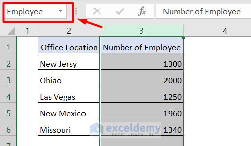
• When we select Column 3, we can see the name Employee.

Read More: How to Edit Named Range in Excel

Download the Practice Workbook

Related Articles

• How to Find a Named Range in Excel
• How to Change Scope of Named Range in Excel
• How to Paste Range Names in Excel
• How to Display Named Range Contents in Excel
• How to Delete All Named Ranges in Excel
• How to Navigate to a Named Range in Excel
• How to Delete Named Range Excel

<< Go Back to Named Range | Excel Formulas | Learn Excel