This is an overview.
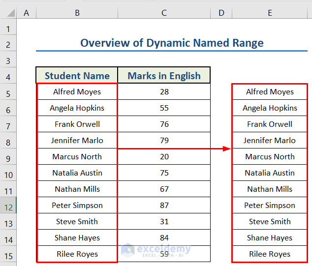
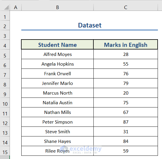
The sample dataset showcases students’ Names and their Marks in English.
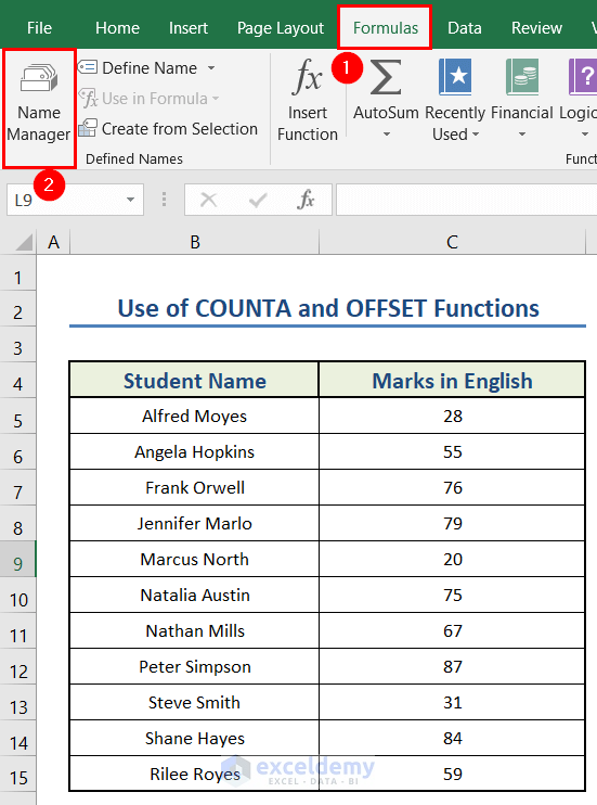
Method 1 – Using the OFFSET Function to Create a One Dimensional Dynamic Named Range in Excel
Steps:
- Go to the Formulas tab.
- Select Name Manager.
- Select New.
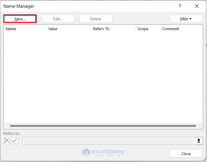
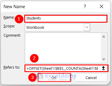
- Enter a Name.
- Use the following formula in Refers to:.
=OFFSET(Sheet1!$B$5,,,COUNTA(Sheet1!$B$5:$B$100))- Click OK.
Formula Breakdown
- COUNTA(Sheet1!$B$5:$B$100)) → counts non-empty cells in B5:B100.
- Output: 11
- OFFSET(Sheet1!$B$5;;;COUNTA(Sheet1!$B$5:$B$100)) → Returns the range of a cell.
- Output: {“Alfred Moyes”;”Angela Hopkins”;”Frank Orwell”;”Jennifer Marlo”;”Marcus North”;”Natalia Austin”;”Nathan Mills”;”Peter Simpson”;”Steve Smith”;”Shane Hayes”;”Rilee Royes”}
- Select E5:E15.
- Enter the following formula in the formula bar.
=Students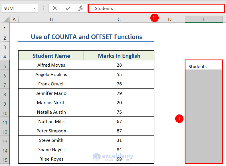
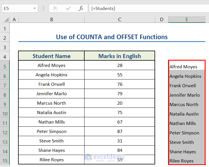
- Press CTRL + SHIFT + ENTER. (It is an array formula)
Excel will show the names in the range.
Note
Read More: How to Display Named Range Contents in Excel
Method 2 – Use the INDIRECT Function to Create a Two Dimensional Dynamic Named Range in Excel
Steps:
- Open the New Name box following the steps described in method-1.
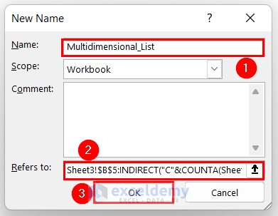
- Set a name.
- Enter the following formula:
=Sheet3!$B$5:INDIRECT("C"&COUNTA(Sheet3!$C:$C)-2+ROW(Sheet3!$C$5))- Click OK.
- Select E5:E15.
- Use the following formula in the formula bar.
=Multidimensional_List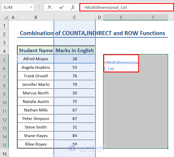
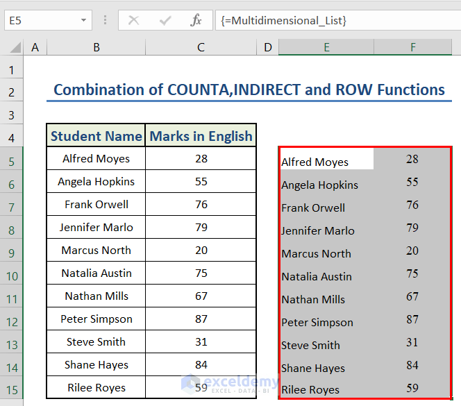
- Press CTRL + SHIFT + ENTER.
Excel will show the names in the range.
Formula Breakdown
- ROW(Sheet3!$C$5) → returns the row number of C5.
- Output: {5}
- COUNTA(Sheet3!$C:$C) → Counts non-empty cells in column C
- Output: 12
- “C”&COUNTA(Sheet3!$C:$C)-2+ROW(Sheet3!$C$5) → The Ampersand (&) joins the texts.
- Output: {“C15”}
- Sheet3!$B$5:INDIRECT(“C”&COUNTA(Sheet3!$C:$C)-2+ROW(Sheet3!$C$5)) → shows the final output.
- Output: {“Alfred Moyes”\28;”Angela Hopkins”\55;”Frank Orwell”\76;”Jennifer Marlo”\79;”Marcus North”\20;”Natalia Austin”\75;”Nathan Mills”\67;”Peter Simpson”\87;”Steve Smith”\31;”Shane Hayes”\84;”Rilee Royes”\59}
Note
Sheet3 is the name of the worksheet.
Read More: Excel INDIRECT Function with Named Range
Download Practice Workbook
Related Readings
- How to Use Named Range in Excel VLOOKUP Function
- Excel Reference Named Range in Another Sheet
- How to Ignore Blank Cells in Named Range in Excel
- How to Use Dynamic Named Range in Excel Chart
<< Go Back to Named Range | Excel Formulas | Learn Excel
Get FREE Advanced Excel Exercises with Solutions!
