Latest Posts From Priti

In this Excel tutorial, you will learn in detail about the mileage calculator in Excel, which includes calculating mileage for vehicles and between cities. ...

Excel's union operation is a potent tool that lets you combine data from various ranges into a single object. Utilizing the Union operator and the ...

In this Excel tutorial, we will show you how to apply alternating row colors in Excel using a manual approach, conditional formatting, table formatting ...

Finding out if time is between range is used to make decisions for attendance tracking, event scheduling, project monitoring tasks, employee shift scheduling, ...

Here's an unsorted pivot table with the annual salaries of each department for different designations and the same pivot table after sorting alphabetically. ...

Download Practice Workbook Copy Chart.xlsx You can copy a chart, with or without formatting, to the same or different worksheets, workbooks, or ...

This is an overview. Download Practice Workbook Create Alerts.xlsm Example 1 - Using the Conditional Formatting to Set Up Alerts When ...

Download the Practice Workbook Import HTML.xlsx Method 1 - Use the Data Tab to Import HTML from Existing Connection Save an HTML file on ...
How to Find All Errors in Excel While working with Excel, some errors are common and occur frequently. Find all errors at once is necessary. Click Find & ...

In this Excel tutorial, you will learn how to apply the number format. You can access number formatting options from the toolbar, ribbon, and number format ...

1 - FV Function (Future Value) The FV function is an Excel financial function that is used to calculate the future value of an investment based on a series of ...

Method 1 - Create Named Range Using Name Box Create a name for the Annual Salary column using the Name Box. Select the cell range F6:F15 >> go to ...

Method 1 - Using the Wrap Text Option from the Home Tab Select range D6:D13. Go to the Home tab. Click on Wrap Text in the Alignment group. ...

In this Excel tutorial, we will review some of the best strategies to make Excel faster with lots of data by avoiding the use of volatile functions, array ...

Excel's Sparklines feature is a helpful tool for identifying data trends. Sparklines are tiny charts that can fit into a single cell and give quick solutions. ...
See Our Reviews at


Hello ZHENG,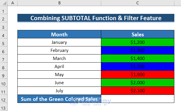
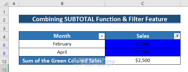
Thank you for taking the time to read our article. If you have cells of different colors (such as green, blue, and red) and want to sum them up, the easiest way is to use the SUBTOTAL function with the Filter command. For example, let’s say you have sales values in the range C5:C11, where cells C5, C7, and C10 are green, C6 and C8 are blue, and C9 and C11 are red.
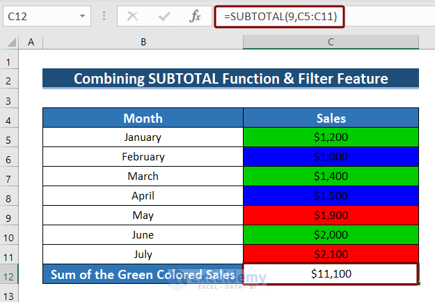
1. To get the sum of a definite colored cell, insert the formula in a cell:
=SUBTOTAL(9,C5:C11)Here, the SUBTOTAL function inserted in cell C12 uses 9 as the “function_name” argument (which refers to the SUM function) and C5:C11 as “ref1”.
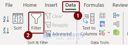
2. Select the column header and go to the Data tab > Sort & Filter > Filter.
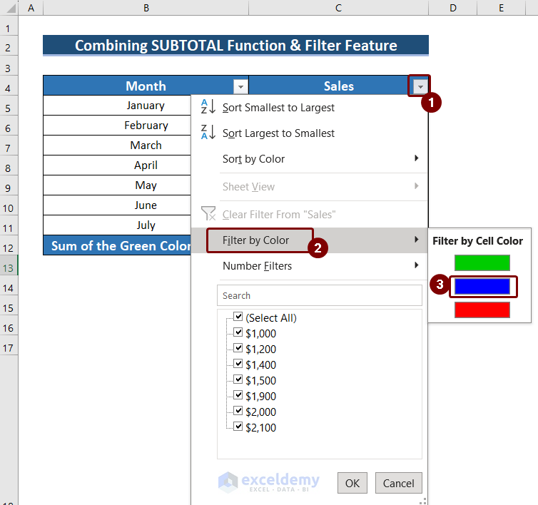
3. Click on the Filter icon of the column and select “Filter by Color.” You will see three different colors to choose from.
4. Select the color you want to sum up, and you will get the sum of all the cells with that color.
You can see the blue-colored cells filtered and summed up.
We hope this helps! Let us know if you have any further questions.
Regards,
Exceldemy Team
Hello DILIP,
Thank you for taking the time to read our article.
In order to automatically copy rows from specific cell ranges without manually selecting them, you will need to include a few lines of code. Here is an example of the code that can be used. Just make sure to adjust the “wsDestination” variable to match the sheet name of your dataset and update the cell ranges in “sourceRange” variable.
We hope this helps! Let us know if you have any further questions.
Regards,
Exceldemy Team
Hello BRANISLAV,
Thank you for reading our article and for your comment.
You can easily create an add-in with the same code mentioned in this article. Kindly follow the steps mentioned below.
1. Copy and paste the code in the article in a Module.
2. Save the Excel file as a Macro Enabled Add-in (.xlam) file. For that, go to the File tab and select Save As.
Select Excel Add-in (*.xlam) from the drop-down under the file name and press Save.
3. Now go back to your Excel file. From the Developer tab, select Excel Add-ins from Add-ins group.
4. Next, Add-ins dialog box will pop up. Browse for the name of your .xlam file, select the checkbox beside it, and press OK. We have chosen Udf_Tooltip as it was the name of our .xlam file.
Now, you can access this UDF in any Excel file on your PC.
Hope this solves your problem.
Regards,
Exceldemy Team
Hello Stefano,
I’m glad you found the information helpful, but I understand you’re still encountering issues with adding the FNC-1 character to your SSCC Code using a Code 128 font.
I apologize for any confusion. The downloaded font here can not directly convert codes into Barcodes. You need to apply the VBA code to create the function “=Code128” to transform the SSCC code into symbols. After that, using the downloaded font will work.
For your second problem, there isn’t a built-in Excel function called “=Code128b” for adding the FNC-1 character. Excel has no native function for generating Code 128 barcodes with special characters.
That is why we built a function named “=Code128” using the VBA code for your convenience. Follow step 2 which is Using VBA to Create User Defined Function to create the function.
I hope the confusion is cleared and this process willwork for you now.
Regards
Exceldemy Team
Hello ALEQ,
Thank you for your query. If you want to sum one specific product of two or three brands you just have to use an OR logic for brands.
Let us assume we want to find the sum of notebook sales of Lenovo and Asus brands. For that insert the following formula:
=SUMPRODUCT(((B5:B21=G12)+(B5:B21=G13))*(C5:C21=G14)*(D5:D21))
Here, (B5:B21=G12)+(B5:B21=G13), this part applies the OR logic for brands. It matches the range B5:B21 with G12 and G13 cell values and returns TRUE or FALSE. So, it returns TRUE for Lenovo and Asus brands and Excel counts them as 1.
Similarly, C5:C21=G14 returns TRUE or 1 for if any match is found and D5:D21 simply returns the sales values.
So, the function sums up the prices of notebooks of two different brands.
If you want to sum up prices for more brands, then just add another logic that matches brands in this part “(B5:B21=G12)+(B5:B21=G13)” of the formula.
Regards,
Priti
Exceldemy Team
Hello WU,
Thank you for bringing that to my attention. You are correct that the proper formula for calculating the approximate yield to maturity (YTM) of a bond is:
YTM = (C + (FV - PV) / n) / ((FV + PV) / 2)I appreciate your attention to detail, and I will ensure to update my article accordingly. Thank you for being a part of our community. If you have any further questions or require assistance, please don’t hesitate to post on our Forum.
Regards,
Priti
Exceldemy Team
Greetings Michal,
Thanks for your comment! I understand the dissatisfaction with the limitations that you’ve faced. I agree that Microsoft could do more to enhance the functionality of their checkboxes.
Regarding your first issue, it is true that the COUNTIF function is unable to directly count the number of checked boxes.
Your second point—that Microsoft does not support Format Control Linking in an array—is also true. This implies that each checkbox needs to be linked separately. This process can take a while, especially if there are a lot of checkboxes.
However, we can do Format Control Linking using VBA code which we already mentioned in this article. Besides, we are adding another code that works as a function and dynamically does format control linking without any helper column and counts the checked boxes.
To work with this code, go to the Developer tab, and select Visual Basic. Now, from the Insert tab >> you have to select Module. Write down the following Code in the Module.
Public Function CheckBoxCount()
Dim checkBox As Shape
Dim count As Long
count = 0
With ThisWorkbook.ActiveSheet
For Each checkBox In .Shapes
If InStr(1, checkBox.Name, “Check Box”) Then
If .Shapes(checkBox.Name).OLEFormat.Object.Value = 1 Then
count = count + 1
End If
End If
Next checkBox
End With
CheckBoxCount = count
End Function
Now, Save the code and go back to Excel File. Insert the following formula in the cell that you want the count of checked boxes.
=CheckBoxCount()
And you will have the count of checked boxes.
Hope this solution helps address your specific requirements in a more efficient manner.
If you have any further queries, kindly post them on our Exceldemy Forum.
Have a nice day!
Regards,
Priti