How to Sort a Pivot Table (6 Easy Ways)

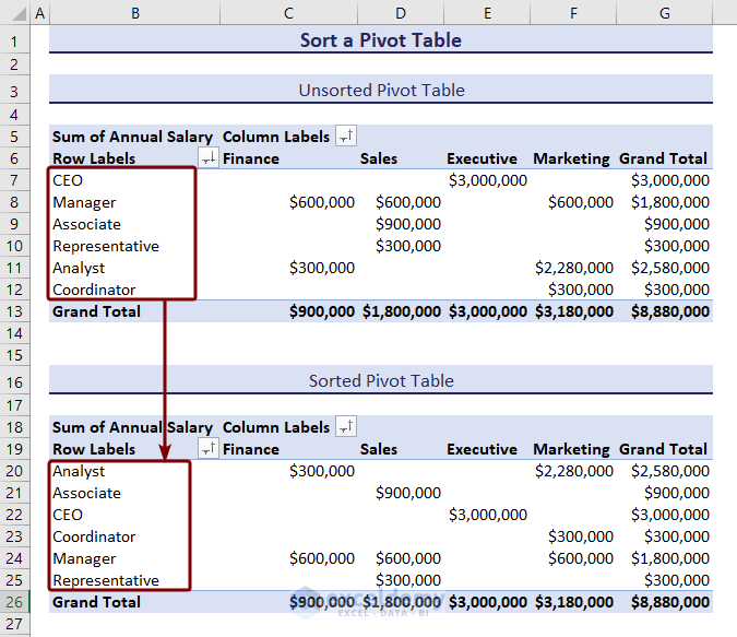
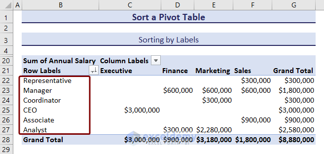
Here’s an unsorted pivot table with the annual salaries of each department for different designations and the same pivot table after sorting alphabetically.

Pivot Table Sorting Restrictions

• If no pivot fields are present to the left of the field you are sorting, all the pivot items will be sorted together in the order you selected.
• If fields are present to the left of the field you are sorting, the pivot items will be sorted within each item of the next field to the left.

6 Ways to Sort a Pivot Table in Excel

We will use the dataset shown below.

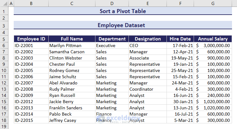
To create a pivot table from this dataset:

• Select any cell in the data range.
• Go to the Insert tab, select PivotTable, and choose From Table/Range.
• In the PivotTable from the table or range box, choose where to put the pivot table in the New worksheet or Existing worksheet and press OK.
• In the PivotTable Fields pane on the right, drag the fields in the Rows, Columns, and Values fields. 

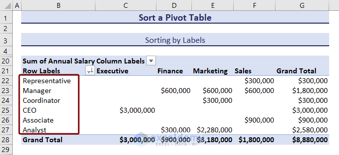
Method 1 – Sorting a PivotTable by Label Data

We want to sort the row labels in the pivot table in alphabetic order.

• Select a cell in the column that is to be sorted by row labels.
• Go to the Data tab and click Sort.
• Choose between Manual, Ascending, or Descending options from the Sort box and press OK.

• We chose the Descending sorting option. You can also sort by values or auto-sort by clicking More Options.

• The pivot table will be sorted in descending order.

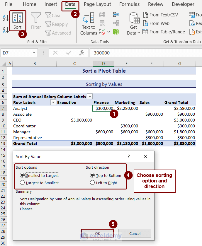
Method 2 – Sorting by Values

• Select a cell with a value in the pivot table.
• Go to the Sort tab and select Sort from the Sort & Filter group.
• In the Sort By Value box:
  • Choose the sorting option, either Smallest to Largest or Largest to Smallest.
  • Choose the sorting direction Top to Bottom or Left to Right.
  • Press OK.

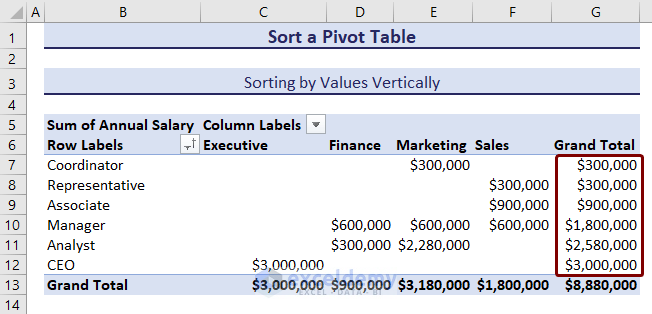
As we can sort pivot tables by values in two different directions, we will sort them vertically and horizontally by the Grand Total values.

Case 2.1 – Sorting a Pivot Table by Grand Total Horizontally

• Select a cell with a Grand Total value horizontally in the pivot table.
• Go to Data and select Sort.
• In the Sort By Value box:
  • Choose Smallest to Largest as sorting option.
  • Choose Left to Right as sorting direction.
  • Press OK.

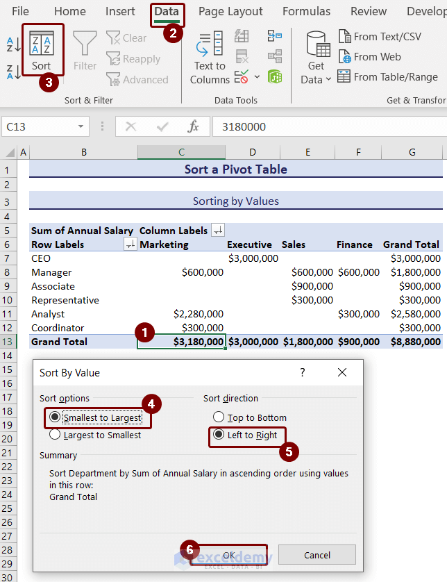
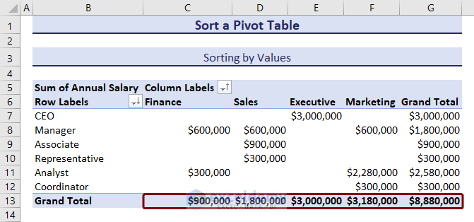
• The Grand Total values in the row will be sorted from smallest to largest.

Case 2.2 – Sorting a Pivot Table Vertically

• Select a cell from the Grand Total column and choose Top to Bottom as sorting directions.

Sorting the grand total in the vertical and horizontal directions can be done concurrently.

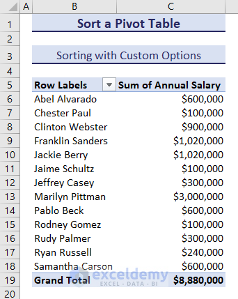
Method 3 – Sorting a Pivot Table with Custom Options

We have a pivot table with employee names and their annual salaries shown in the image below.

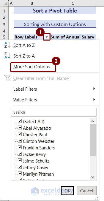
• Click on the filter arrow for Row Labels.
• Select More Sort Options.
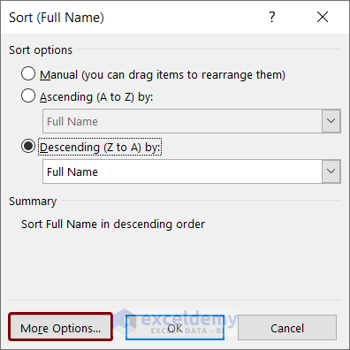
• In Sort box, choose Manual, Ascending, or Descending. We chose Descending option.
• Press More Options to see more sorting options.
  
• In the More Sort Options box, check AutoSort and press OK.
  

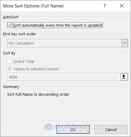
AutoSort will automatically sort every time the report is updated. If you uncheck this option, the First key sort order option will be available, and you can choose a custom order to sort. In general, you can see the weekdays and months in a year as a custom list. However, you can also create your own custom sort list and use that list from here. Updating (refreshing) the data in your PivotTable results in the loss of the sorting order.

• In the Sort By feature, select either Grand Total or Values in specific columns to arrange the data based on these values. This functionality is disabled when the sorting is set to Manual.

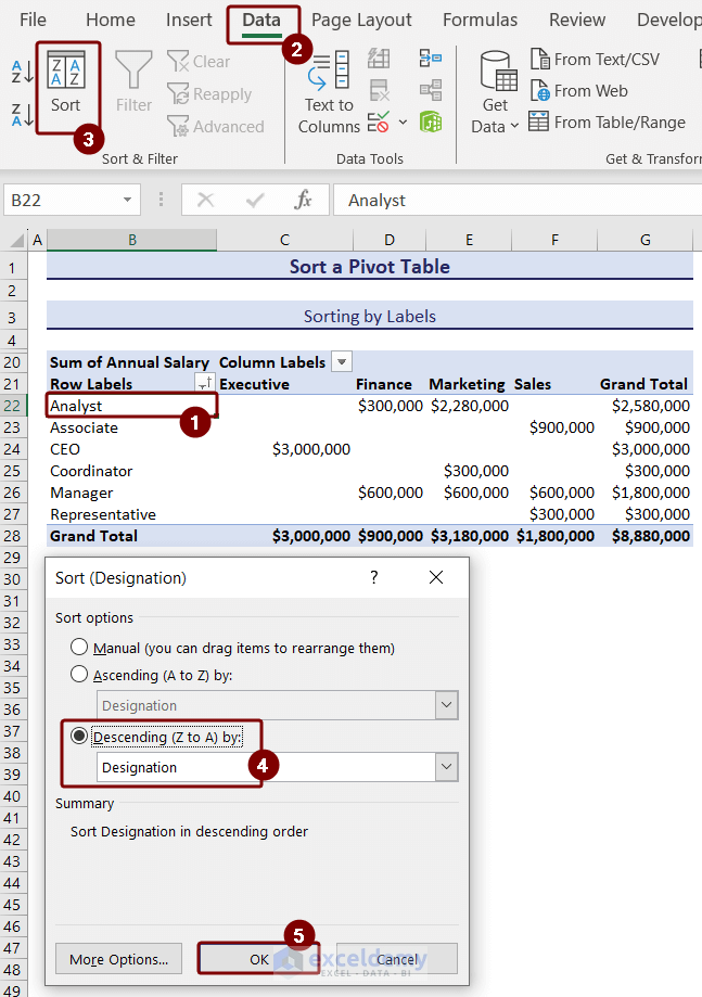
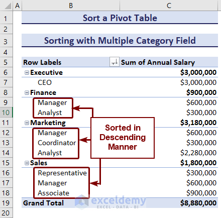
Method 4 – Sorting a Pivot Table with Multiple Category Fields

We have a pivot table that shows annual salaries for different departments.

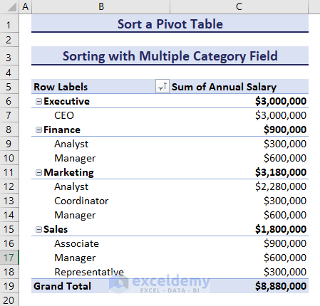
While sorting by row labels, this pivot table will sort by department. Let’s sort by employee designations:

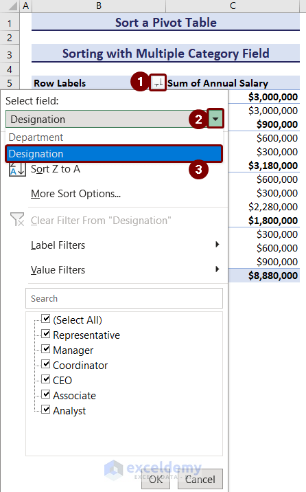
• Click on the sort and filter sign for Row Labels.
• Click on the drop-down for Select Field.
• Choose the category field or row label to sort. We chose Designation.

• Select the sorting option. We selected the “Sort Z to A” option.
• Press OK.
  

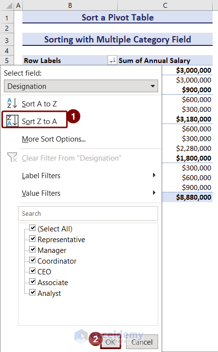
After sorting, the designations of each department will be sorted in a descending order.

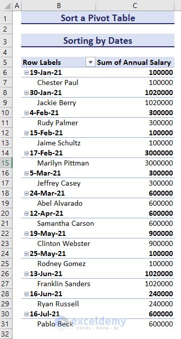
Method 5 – Sorting a Pivot Table by Dates

We have a pivot table containing the employee names, their hiring dates, and annual salaries.

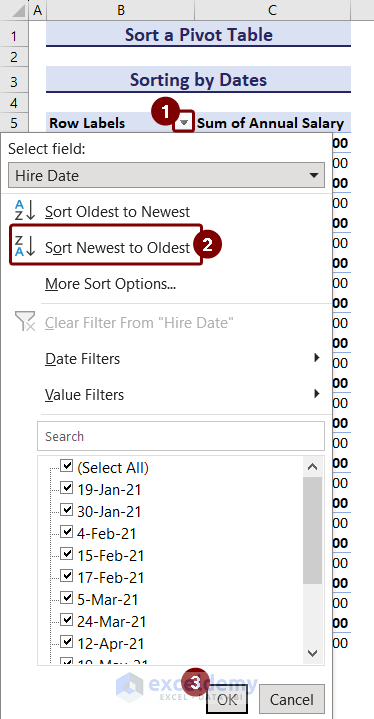
• Click on the sort and filter sign for Row Labels.
• Select the Sort Newest to Oldest sort option.
• Press OK.

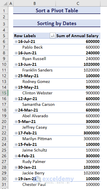
• The dates are sorted from newest to oldest in the image below.

Method 6 – Sort Pivot Fields with a Macro

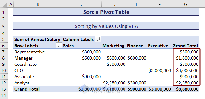
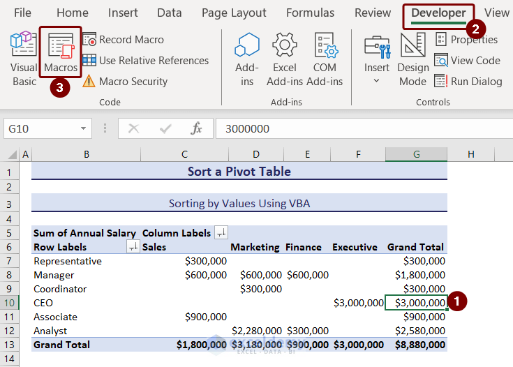
We will sort the Grand Total column of the pivot table in ascending order using VBA.

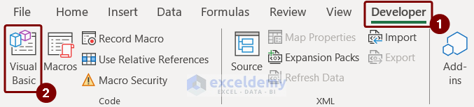
• Go to the Developer tab and select Visual Basic.
  
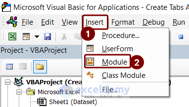
• Go to Insert and select Module in the Microsoft Visual Basic for Applications window.
  
• Insert the following VBA code in the module.

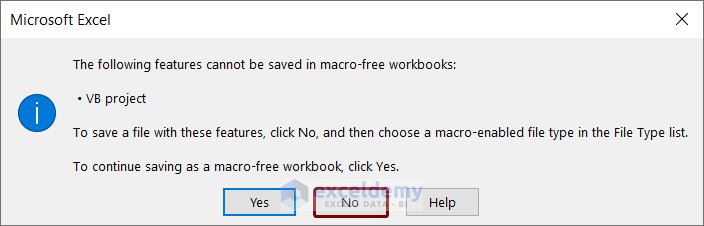
  Sub SortUsingVBA()
      ActiveSheet.PivotTables("PivotTable4").PivotFields("Designation").AutoSort _
          xlAscending, "Sum of Annual Salary", ActiveSheet.PivotTables("PivotTable4"). _
          PivotColumnAxis.PivotLines(5), 1
  End Sub

• Press Ctrl + S to save the file as a macro-enabled file.
• Click the No button in the Microsoft Excel dialog box.
  
• In the Save As dialog box, choose the Save as type option as .xlsm type and click the Save
• Go back to the sheet and select a cell in the column to sort.
• Select Macros from the Code group in the Developer tab.
  
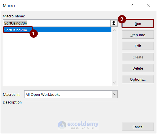
• Select the SortUsingVBA macro and click on the Run button in the Macro box.
  
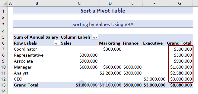
• You can see the pivot table is sorted by values in ascending order.

What to Do If Pivot Table Sorting Is Not Working in Excel?

Case 1 – Pivot Table Sort by Value Not Working

The image below shows that the grand total of annual salaries for each designation column is sorted in ascending order. But the Finance column is not sorted in ascending order.

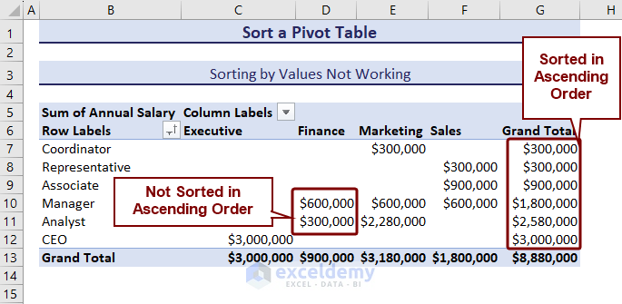
Reason:  The pivot table makes groups of different parts of data. When the pivot table is sorted based on grand totals, all the designations are sorted based on that value. However, the finance department’s column can not be sorted similarly as it will disrupt the existing order. The pivot table gets filtered based on the value of the right-most column. Also while sorting it does not take any other column on the left of that in considertaion.

Solution: Decide which column value you want to consider for sorting your data. Put that column as the rightmost column of your pivot table.

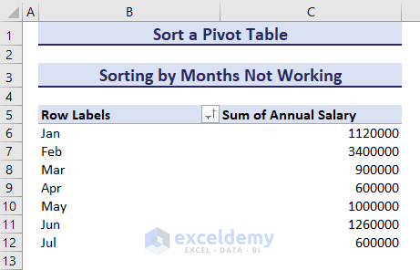
Case 2 – Pivot Table Months Not in Order

The pivot table might sort the months alphabetically, like in the image below.

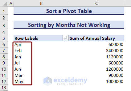
Reason: Pivot table sorts months with a default custom sort list of months. If this custom sorting is disabled, then months get sorted alphabetically.

Solution:

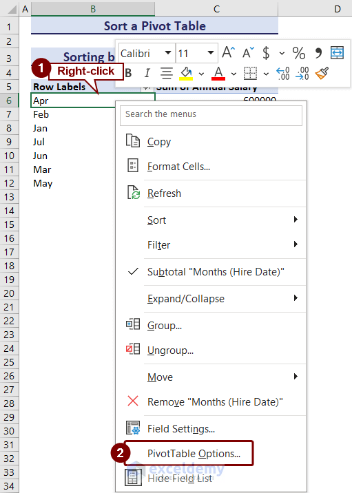
• Right-click on any cell in the pivot table.
• Choose PivotTable Options from the context menu.
  
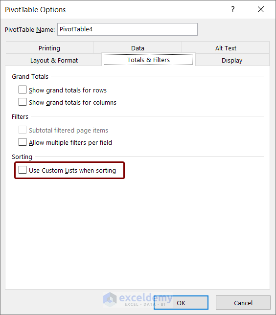
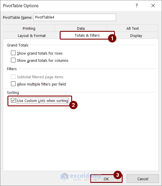
• In the PivotTable Options box, go to the Totals & Filters section.
• Under Sorting, check Use Custom List when Sorting.
• Press OK.
  

You will see the months automatically sorted in custom order instead of alphabetically sorting.

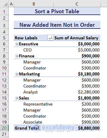
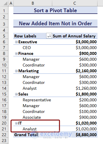
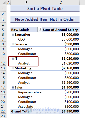
Case 3 – New Pivot Table Items Out of Sort Order

We have a sorted dataset showing annual salaries for different designations of each department.

We added a new department named “IT” with “Analyst” designation. After refreshing the pivot table, the “IT” department was added at the bottom.

Solution:

• Click on the Row Labels sort and filter sign.
• Choose the Sort A to Z option and press OK.
  

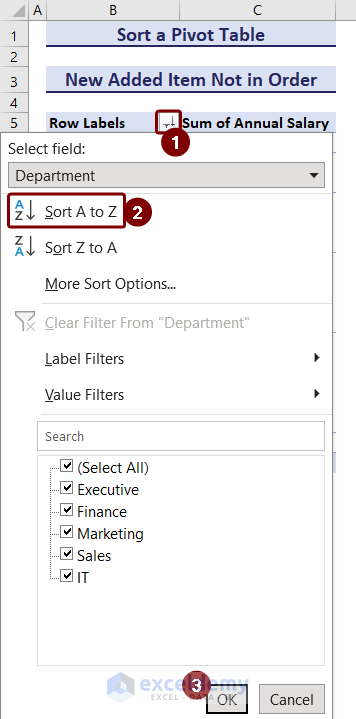
You will find the list sorted in the proper order.

Frequently Asked Questions

Why Does Excel Not Allow Sorting?

Excel can sort most of the data sourced externally. However, Excel can not sort data sourced externally from an SQL table or some other sources. In this case, you have to copy and paste the data as value in your spreadsheet and then use pivot table sorting.

Why Pivot Table Report Filter Is Not Sorted?

If new data is added to the source data and after refreshing it is not shown as a sorted list in the pivot table report filter. In this case, drag that category from the filter field into the Value field so that pivot table can treat it as a value field. Then apply sorting and drag the field again to filter the field. Now, you can see the newly added items in sorted order in the report filter.

How to Sort Pivot Table by Count?

To sort the pivot table by count, click on the arrow sign of a value field, select Value Field Settings, choose Count from the Summarize value field by section, and press OK. Now when you sort that value field column, it will be sorted based on the count value.

<< Go Back to Pivot Table in Excel | Learn Excel