Excel is frequently used in finance, accounting, data analysis, and project management. However, if there is any error in formulas, that can hamper your work. So, to ensure accurate calculations and error-free work, it is essential to know why the formula errors occur and how to resolve the issue. Therefore, in this article, I will show you 10 common Excel formula errors that occur frequently in Excel, along with the reason and solution of them.
Download Practice Workbook
You can download the practice workbook here.
How to Find All Errors in Excel
While working with Excel, some errors are common and occur frequently. So, to avoid them, knowing how to find all errors at once is necessary. Click Find & Select, then select Go To Special… from the Home tab. Or you can use the keyboard shortcut Ctrl+G and select Special from Go To box.
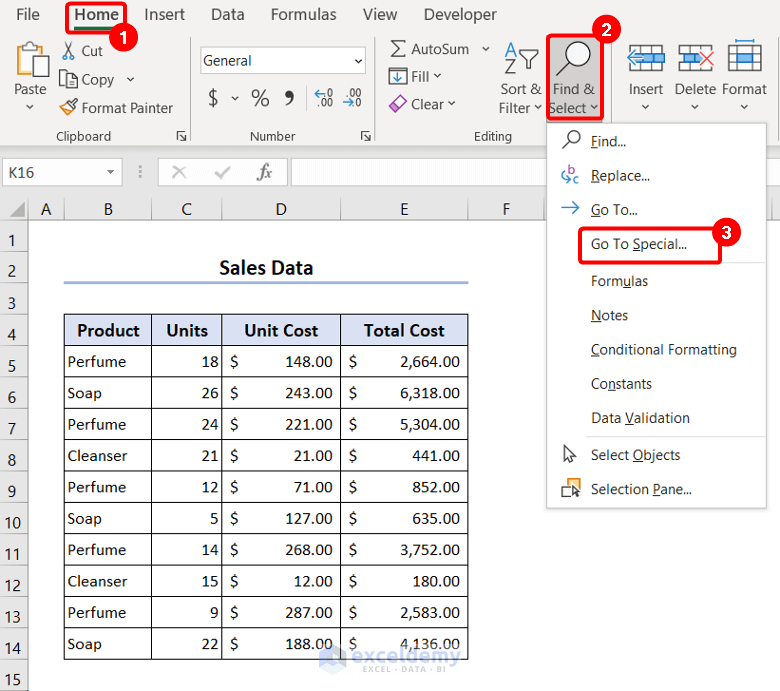
From the Go To Special box, check only the Errors option in the Formula section to find only the Formula Errors.
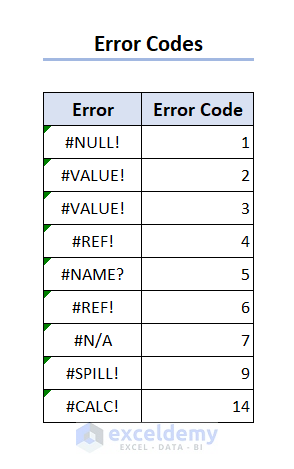
Error Codes
Each error contains an error code that can be found using ERROR.TYPE function. Below there is a list of these error codes.
#NULL! : 1
#DIV/0! : 2
#VALUE! : 3
#REF! : 4
#NAME? : 5
#NUM! : 6
#N/A : 7
#SPILL! : 9
#CALC! : 14
10 Common Formula Errors with Reason & Solution
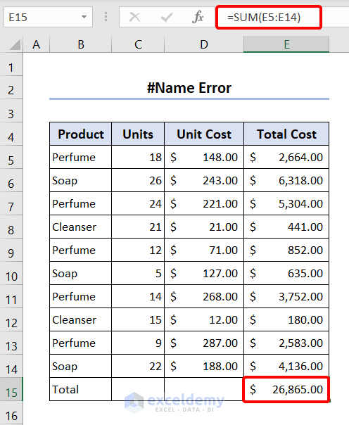
To demonstrate different formula errors, I have a dataset containing a company’s sales data. Here, I have the product name, units sold, unit cost, and total cost of each product.
Now, I will show you the reasons and solutions for the 10 most common formula errors in Excel using this dataset.
1. #NAME? Error
Invalid name error, #NAME? , occurs when Excel does not recognize something, i.e., a function name, a misspelled function name or named range, cell reference not matching, etc. For example, in the image below, I wanted to calculate the sum of total costs. But I misspelled the function name resulting in #NAME? error.
Solution:
To solve this error, insert the function name properly. Select the cell where the formula was before, enter the right formula carefully, and you will see the error removed.
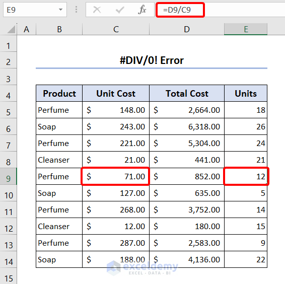
2. #DIV/0! Error
#DIV/0! or divided by zero occurs when a value is divided by zero. Since any value divided by zero is undefined, Excel shows an error. In the image below, you can see no value in cell C9, meaning it contains 0. So, when I tried to divide the value of D9 by C9, Excel returned a #DIV/0! error.
Solution:
Insert a numerical value instead of 0. Here, I inserted $71.00 as the unit cost of perfume, and we can see the unit amount instead of the error value.
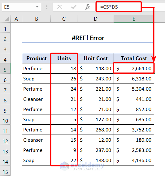
3. #REF! Error
#REF! Error is a common error. Excel shows it if any cell reference is invalid.
Like in the image below, I calculate the total cost by multiplying Units and Unit Cost values. Now I will delete the Units column by selecting it and clicking Delete Sheet Columns from the Delete drop-down.
Next, you will see that the Total Cost column contains #REF! Error as cell references of the Unit column is invalid now.
Solution:
So, to resolve this error, you need to check if the cell reference is valid and then change it accordingly. Moreover, before deleting or making any change in your Excel sheet, ensure all the formulas are pasted as values to prevent this error.
As I inserted the Units column here, the errors are removed now.
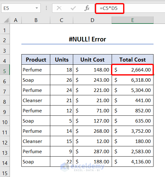
4. #NULL! Error
#NULL Error occurs if there is a typo in the formula, such as a space inserted instead of a comma or colon.
For example, an asterisk sign was supposed to be between the cell references in the image. Instead, a space was inserted, resulting in a #NULL error.
Solution:
Avoiding typos or being careful while inserting formulas is the key to solving this error. Here, I inserted the corrected formula and got the desired result.
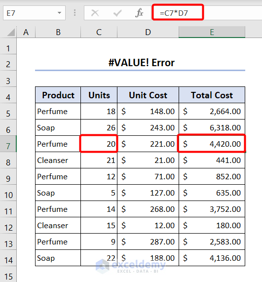
5. #VALUE! Error
When a value is not inserted in an expected or valid format (Number, text, time, date, etc.), #VALUE! error occurs. For example, if a text value is entered where a numeric value is expected, a cell is left blank, or dates are formatted as text.
As you can see, I entered the unit value as “twenty,” whereas it should have been “20,” resulting in #VALUE! error.
Solution:
Insert the properly formatted value and check the valid type of value while inserting the value to avoid this error. Here, I inserted a numeric value to avoid the #VALUE! error.
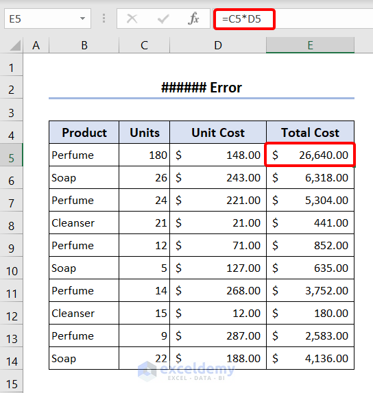
6. ###### Error
###### error is common though it technically is not an error. You will see most often, after inserting a formula, Excel displays a string of hash signs (####) instead of the output. This happens if the value in the cell is too wide to fit in the column.
Here, the value in cell E5 does not fit in the column width it currently is in, thus showing a #### error.
Solution:
The solution to this error is to widen the column. To do that, drag the column handle showing the ##### error and pull it to the right side until the error disappears and values appear, or double-click on it to adjust the width.
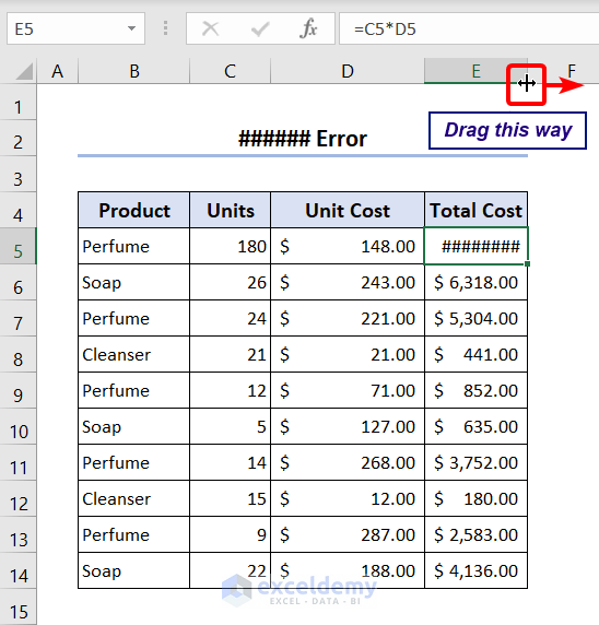
Here, the error disappeared as I increased the column width.
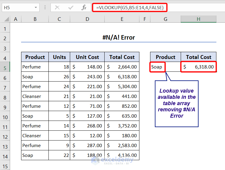
7. #N/A Error
The #N/A error appears when Excel cannot locate something, i.e., a misspelled name or function, extra spaces, etc. VLOOKUP, LOOKUP, HLOOKUP, and MATCH functions are impacted mainly by #N/A errors, as an incomplete lookup table is one of the most common reasons for the not available error.
For example, look at the image below; here, I was trying to find the total cost for “Hand Wash”, but this product name does not match the product names in the table array. So the lookup function shows the #N/A error.
Solution:
To avoid the #N/A error, check if the lookup value is available in the table array while working with LOOKUP functions, and for other cases, check for any misspelling or extra space characters.
In my case, I entered “Soap” as a product name instead of “Hand Wash” since the values for “Soap” are available in the table array.
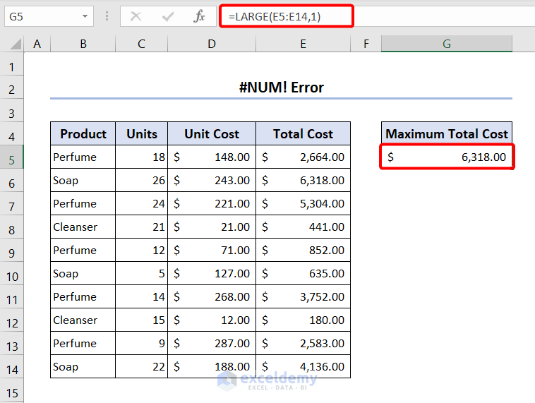
8. #NUM! Error
The #NUM error occurs if the calculated output is either too small, too large, or impossible to calculate, i.e., the square root of the negative number.
Here, the LARGE function is applied to calculate the maximum total cost. But the rank of the large number entered is 11 instead of 1, which caused the #NUM error. So, here the formula mainly tries to find out the 11th large number from the range, which is not possible as there are only 10 entries resulting in a #NUM error.
Solution:
The solution to this error is to apply them properly so that the function can calculate properly. I replaced 11 with 1 to find the maximum total cost in the LARGE function.
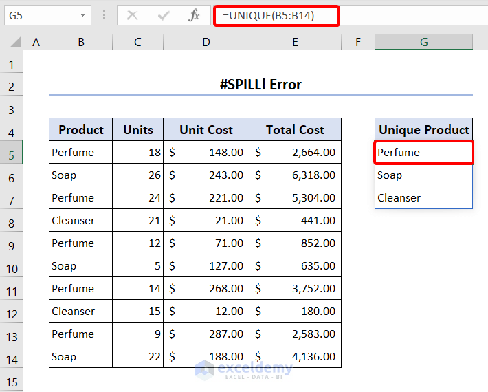
9. #SPILL! Error
In Excel, some functions return spill range, mainly a set of cells containing the output. If these functions run into any entry in a cell where the result was supposed to be entered, then a #SPILL! error occurs.
Like, the UNIQUE function finds the unique product names, which are three in number. So this function needs three cells for displaying the output, but it encounters an entry “John” in the second cell. As a result, it shows #SPILL! error.
Solution:
To avoid this error, check if there is any entry in the adjacent cells of the cell where you are applying a formula that will return a spill range. Also, if a #SPILL! error appears, then check which cell entry is hindering the function from working, select the cell, and press the Delete button.
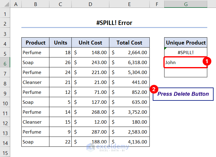
Finally, the #SPILL! error will disappear, and you will see the desired outcome.
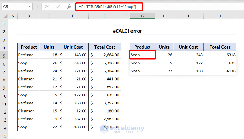
10. #CALC! Error
While applying a formula that works with an array, if the formula cannot calculate because of misinformation or anything else, then a #CALC! error occurs.
For example, the FILTER function filters the values from the range B5:E14 if B5:B14 matches “Hand Wash.” However, in cell range B5:B14, there is no “Hand Wash” entry, which does not let the FILTER function calculate, resulting in a calculation error.
Solution:
The solution to this error is to be cautious while working with the functions that give output in an array. I inserted “Soap” as the product name, which matches the range B5:B14 and filters all the entries of the mentioned product.
Things to Remember
- To avoid formula errors while working, you can use the IFERROR function.
- ##### error does not contain any error code as it is not an error technically. It simply says that you need to widen your columns to make the output visible.
Conclusion
This article demonstrated the reasons and solutions for 10 common Excel formula errors. In addition to that, it also showed how to find all errors easily using the Go To Special option. Furthermore, it also provided a list of error codes in Excel. Excel formula errors help you make your calculations consistent and error-free. So, knowing about them is necessary for working efficiently in Excel. Lastly, I hope this article taught you why and when the Excel formula occurs and how to handle them efficiently.
Frequently Asked Questions
1. How do I turn off formula errors?
If you do not want formula errors to show up, then you can turn them off. To do that, select Options from the File tab. In the Excel Options box, select Formulas from Error Checking section, and uncheck the Enable background error checking check box.
2. How to Find Errors with Automated Error Checking?
By default, Excel highlights some formula errors displaying a green triangle on the top left side of a cell. Click on the triangle, and you will see the explanation of the error.
3. What is an error in Excel formula ####?
Excel shows a #### error if the column width cannot display
Excel Formula Errors: Knowledge Hub
<< Go Back to Errors in Excel | Learn Excel
Get FREE Advanced Excel Exercises with Solutions!