Latest Posts From Nujat Tasnim

Here's an overview of the Equations Editor in a cell. Download the Practice Workbook Equation Editor.xlsx What Is the Equation Editor ...

We will use the following sample dataset to insert quotes in various cells. Download the Practice Workbook Use of Quotes.xlsm What Is ...

Method 1 - Machine Learning Algorithm Step-1: Prepare Training Data To demonstrate the whole procedure, we have taken the following sample dataset, which ...

Here's an overview of a simple IF check that returns a predetermined pair of values. Download the Practice Workbook Cells Containing Text.xlsx ...
Method 1 - Encrypt an Excel File Using Encrypt with Password Feature Go to File>> Info>> Protect Workbook>> Encrypt with Password. ...

Method 1 - Use ‘Open as Read-Only’ Feature to Make Excel File Read Only Go to File>> Info>> Protect Workbook>> Always Open Read-Only. ...
In this Excel tutorial, we provide a comprehensive look at ANOVA in Excel. We will demonstrate how to enable the Data Analysis feature and use it to perform ...
Dataset Overview Assume we have a dataset with two worksheets: Sales Record of Year 2021 and Sales Record of Year 2022. Both worksheets contain 7 rows and 3 ...

In this Excel tutorial, you will learn everything about adjusting and changing cell size in Excel. Here's an overview of one of the 10 methods we'll discuss. ...

In this Excel tutorial, we will learn about critical value in Excel. First, we will discuss what is critical value and the different types of critical value. ...

Step 1 – Create Formation of an Initial Balance Sheet Take into account every expense of the business and organize them. We have organized the ...

This is the sample dataset. Download Practice Workbook You can download the practice workbook and the PDF file: PDF to Excel.xlsx ...
Download Practice Workbook Use of Name Manager.xlsx What Is Name Manager in Excel? Name Manager in Excel is used to create, modify, ...
This is an overview. Download Practice Workbook Download the practice workbook here: Here's the password- 12345. Protecting Workbook.xlsm ...
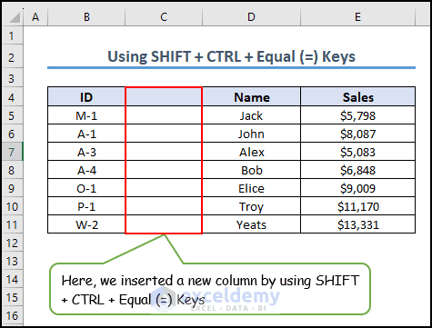
This is an overview: Download Practice Workbook Download the practice workbook. Inserting Column.xlsm This is the sample dataset. ...
See Our Reviews at


Hi NISHANT,
Thank you for your comment. We are sorry that the provided possible solutions aren’t working for you. Before discussing the issue I want to remind you that the Stocks and Geography command under the Data Types tab is only available in Microsoft Office 365. The Data Type tab under the Data ribbon is not available except for Microsoft Office 365.
First, let me mention the three conditions that you must fulfill to show the Data Type tab.
● Need to be an Office 365 Subscriber.
● Editing Language should be set to English.
● Need to sign in to the Office application with your Office 365 account.
Note: You will not be able to use the Data Type tab under the Data ribbon when offline.
Please check whether all three conditions are met. I hope you can solve your problem by fulfilling three conditions and following the three solutions mentioned in the article.
If you haven’t solved the problem yet, here are some other ways that might help you to solve the issue.
● Check for Updates: Make sure your Office 365 applications are up-to-date. In many cases, Microsoft releases updates and bug fixes on a regular basis, so updating your software may resolve the problem.
● Check Add-ins: Sometimes third-party add-ins cause problems. Ensure no unnecessary add-ins are enabled and restart Office.
● Create a New User Profile: Often, issues are related to user profiles. Try creating a new user profile on your computer and see if the issue persists.
You can also provide us with the version information. Also, I would appreciate it if you would upload a screenshot of your Data tab so we can better understand your exact scenario and give suggestions in a productive manner. Please feel free to reach out to us with any other questions.
Regards
Nujat Tasnim
Exceldemy.
Hi JASON,
Thank you for your comment. According to your comment, I understand that you want to alter the code so that you don’t have to choose a worksheet but instead, it enters new data on the worksheet you are currently on.
For this, you don’t need any ListBox named ListBox1. Follow the below steps:
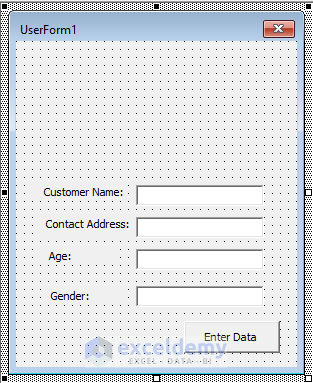
● In Step 1, while developing the UserForm to create the Data Entry Form, you don’t need to put ListBox1 as there will be no selection option according to your query.
So the UserForm will look like the following image.
● Now, in Module 1 insert the following code and save it.
Sub Run_UserForm()
UserForm1.Caption = “Data Entry Form”
Load UserForm1
UserForm1.Show
End Sub
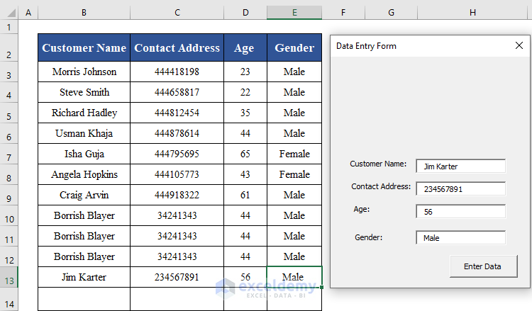
Now, you are good to go. You will not have to choose a worksheet instead, it enters new data on the worksheet you are currently on.
Here is a sample image. I have entered data in the worksheet named Washington.
Hopefully, you will be able to solve your problem now. Please feel free to reach out to us with any other questions or you can send us your Excel files as well.
Regards
Nujat Tasnim
Exceldemy.
Hi AHMED KAMEL,
Thank you for your comment. According to your comment, I have understood that you want to generate random numbers in a range with Excel VBA by defined number and distribute 100 random numbers on 20 cells whereas the total sum of these cells is 100.
To solve this issue follow the below steps:
● Insert a new module and copy and paste the following code.
● Now, run the macro by pressing F5.
This code will distribute 100 random integers across 20 cells in such a way that their sum equals 100. The random number range is specified by minValue and maxValue. Here is the final output image after running the VBA macro successfully.
Change the sheet name according to yours. You can download the Excel file below.
https://www.exceldemy.com/wp-content/uploads/2023/08/Answer.xlsm
Hopefully, you will be able to solve your problem now. Please feel free to reach out to us with any other questions or you can send us your Excel files as well.
Regards
Nujat Tasnim
Exceldemy.
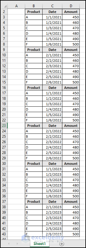
Hi BICKY,
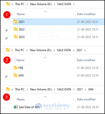
Thank you for your comment. According to your comment, I understand that you have a folder named SALE DATA and in that folder, you have another 3 folders named 2021, 2022 and 2023. Each sales year folder has two folders (JAN, and FEB) and then an Excel workbook. You want to collect sales data from all 3 years in a single workbook.
To solve this issue follow the below steps:
● Insert a new module and copy and paste the following code.
● Set the base folder path and the target sheet where you want to collect the data according to your PC.
● Run the macro by pressing F5.
You can see that the macro successfully extracted data to the new worksheet. You can download the Excel file below.
Answer.xlsm
Hopefully, you will be able to solve your problem now. Please feel free to reach out to us with any other questions or you can send us your Excel files as well.
Regards
Nujat Tasnim
Exceldemy.
Hi BLA,
Thank you for your comment. I think your concern lies in Method 2. In Method 2, we have used the Range.Copy method of Excel VBA to copy without a clipboard. The syntax of this method is given below:
This method does not copy to the Clipboard if the Destination argument is assigned. If this argument is deleted, Microsoft Excel copies the range to the Clipboard. In Method 2, we have used the Destination argument.
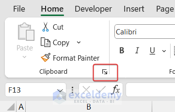
Moreover, you can check the Clipboard after running the code to see if it is using the Clipboard or not.
To check, go to the Home tab and click on the down-arrow beside the Clipboard option.
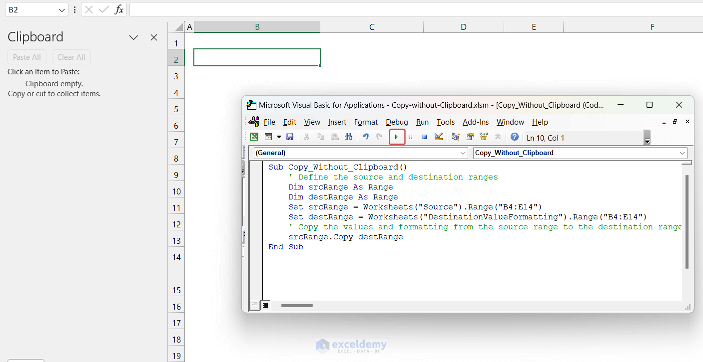
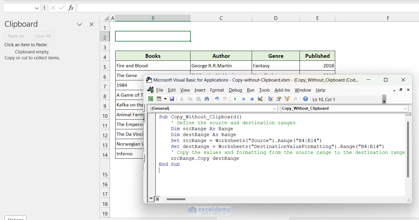
Keeping the clipboard open, we ran the VBA code again.
As you can see, the clipboard shows nothing on it after running the VBA code successfully.
If you copy something in Excel, the clipboard will display the values. Hopefully, this answer will clear your confusion. Please feel free to reach out to us with any other questions or you can send us your Excel files as well.
Regards,
Nujat Tasnim
Exceldemy.
Hi LESLIE,
Thank you for sharing your valuable feedback. We appreciate it very much. I understand your confusion. It is possible that a cell appears to be empty but the ISBLANK function returns FALSE for one of these 3 reasons:
● A regular space is present in the cell.
● A non-breaking space is present in the cell.
● It contains a zero-length string.
A zero-length string, also known as an empty string, is a string with zero characters; as a result, when a cell contains a zero-length string, the LEN function returns 0. In Excel, both blank and empty cells appear empty; however, blank cells include a formula or value that evaluates to or represents a zero-length string, but empty cells do not.
In this image, you can see that cell C7 appears blank, but it’s not! It contains a zero-length string created by entering a single apostrophe (‘) and formatted like other values: General.
You can find out the Excel cells which contain zero-length strings by applying the following formula:
● Insert the following formula in cell D5 and press Enter.
● Now AutoFill the rest of the column’s cells to apply the same formula.
=IF(AND(LEN(C5)=0,NOT(ISBLANK(C5))),"Zero-length string","Not a zero-length string")After that, you can remove the zero-length strings manually. Just select the cells and press the Delete key. Then sort to get the desired output.
Hopefully, you will be able to solve your problem now. Please feel free to reach out to us with any other questions or you can send us your Excel files as well.
Regards,
Nujat Tasnim
Exceldemy.
Hi AIDAN,
Thank you so much for sharing your valuable feedback. We appreciate your participation and are available to assist. I assume you wish to display page numbers at the top of your Excel spreadsheet. The following VBA code may solve your particular problem:
1. First, follow the first 3 steps from Method 1.
2. After that, type the following code in the module.
3. Now open the Macro dialog box: Developer > Macros.
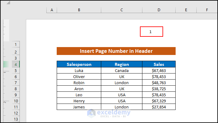
4. Select the specified Macro name which is Page_Numbers_inHeader and press Run.
5. You will see the macro has inserted the page number in the header.
Hopefully, you will be able to solve your problem now. Please feel free to reach out to us with any other questions or you can send us your Excel files as well.
Regards
Nujat Tasnim
Exceldemy.
Hi BELINDA H,
Thank you for sharing your valuable feedback. We appreciate it very much. First of all, I apologize for the inconvenience. This code worked perfectly when I ran it again. But based on your query, we have identified some possible reasons for this error.
The error you’re encountering in the line Set sWB = Workbooks.Open(Filename:=CurrentF) is likely due to an issue with the file path or the file itself. There are a few possible reasons for this error:
1. Incorrect File Path: Ensure that the CurrentF variable contains a valid file path. Double-check that the file path is correct and that the file exists at that location.
2. File in Use: If the file you’re trying to open is already open in another instance of Excel or by another user, you may encounter an error. Make sure the file is not being used by another process.
3. File Format Compatibility: The code is designed to open Microsoft Excel workbooks with the extensions .xls, .xlsx, or .xlsm. If you’re trying to open a file with a different extension or a file that is not a valid Excel workbook, you may encounter an error. Ensure that the file you’re trying to open is in a compatible format.
4. Security Settings: If your Excel application has certain security settings enabled, such as macro security or protected view, it may prevent the opening of certain files. Check your Excel security settings and make sure they allow for opening files from the specified location.
By troubleshooting these possibilities, hopefully you should be able to identify the reason behind the error and resolve it accordingly. Please feel free to reach out to us with any other questions or you can send us your Excel files as well.