The following sample dataset will be used for illustration.

⏷ Apply Conditional Formatting to Compare Tables and Highlight Differences
⏵ Use Unique Feature to Compare Two Tables
⏵ Use Formula to Compare Two Tables
⏷ Apply VBA to Compare Two Tables and Highlight Differences
⏷ Apply Power Query to Compare Two Tables and Merge All Values
⏷ View Two Tables Side by Side in Excel to Compare Them
⏷ Steps to Compare Two Pivot Tables
⏵ Create Two Pivot Tables in One Sheet
⏵ Insert the Formula to Calculate Differences Between Pivot Tables
⏷ Frequently Asked Questions
⏷ Compare Tables in Excel: Knowledge Hub
Method 1 – Apply Conditional Formatting to Compare Tables and Highlight Differences in Excel
You can apply the built-in unique feature or a custom formula to compare tables and highlight the differences. In the custom formula, you can use the Not Equal (“<>“) operator or the COUNTIF function.
1.1 Using Unique Feature to Compare Two Tables
- Select full table cell range B4:F10.
- Go to the Home tab >> Conditional Formatting >> Select New Rule.
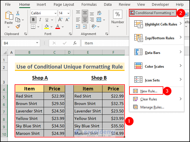
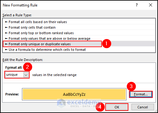
- Select “Format only unique or duplicate values” from the Rule Type section under the New Formatting Rule dialog box.
- Select “unique” from the Format all section.
- Choose a background color using the Format button and click OK.
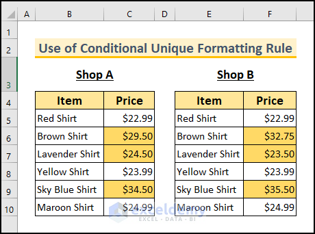
The differences between the two tables are highlighted.
1.2 Using Formula to Compare Two Tables
We can use the Not Equal (“<>”) operator or the COUNTIF function in the Conditional Formatting formula to compare two tables.
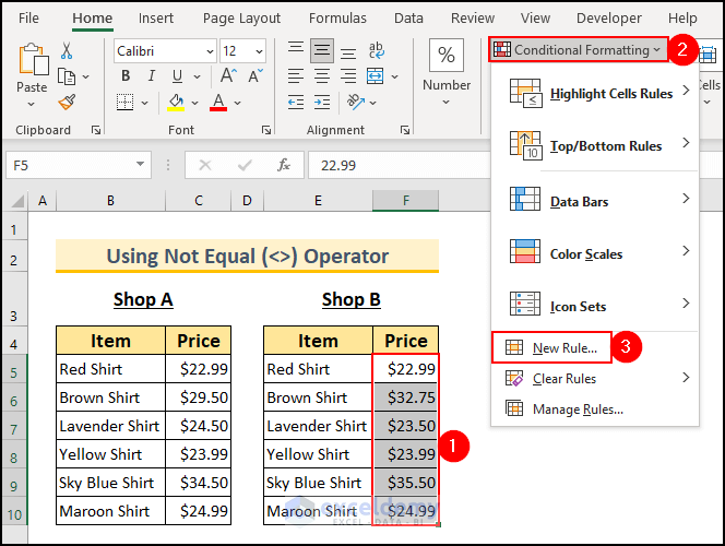
Using Not Equal (“<>”) Operator
- Select cells F5:F10.
- Go to the Home tab >> Conditional Formatting >> Select New Rule.
- Select “Use a formula to determine which cells to format” under the Select a Rule Type section from the New Formatting Rule dialog box.
- Enter the following formula in the Edit the Rule Description box and click on Format.
=F5<>C5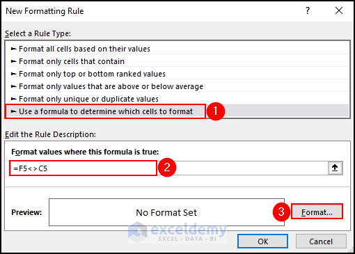
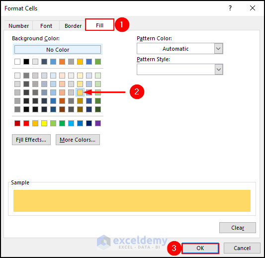
- Select a color from the Background Color section under the Fill tab.
- Click OK.
- Click on OK.
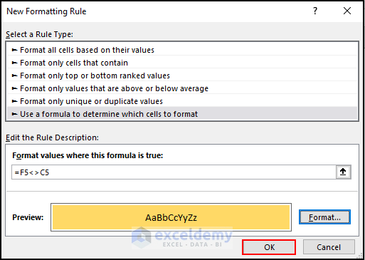
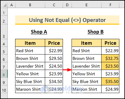
The differences are highlighted as shown below.
Using COUNTIF Function
The COUNTIF function counts the number of cells within a range that meet the given condition. The syntax of this function is given below:
=COUNTIF(range, criteria)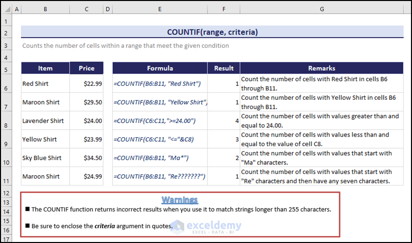
Click the image for a detailed view
- Select cell range C5:C10.
- Go to Home tab >> Conditional Formatting >> Select New Rule.
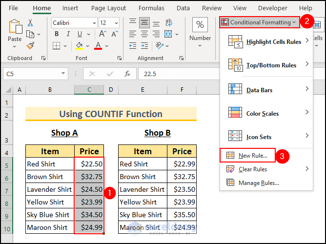
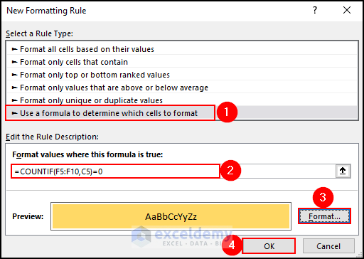
- Select “Use a formula to determine which cells to format” from the Select a Rule Type section under the New Formatting Rule dialog box.
- Enter the following formula in the Edit the Rule Description box.
=COUNTIF(F5:F10,C5)=0- We are checking if our value from the C column is in the F We’ll get 0 if it’s not there.
- We will format the cells that are not in the F5:F10 range.
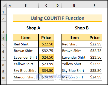
- Choose a background color from the Format section and click OK.
The two tables will be compared and the differences will be highlighted as shown below.
Method 2 – Apply VBA to Compare Two Tables and Highlight Differences
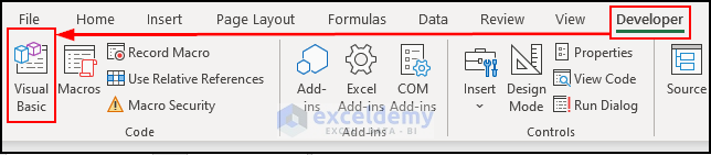
- From the Developer tab >> select Visual Basic.
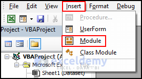
- Select Module from the Insert tab.
- Insert the following code in that module.
Sub HighlightDifference()
Dim i As Long
    For i = 1 To Cells(Rows.Count, "C").End(xlUp).Row
        If Cells(i, "C") <> Cells(i, "F") Then
            Cells(i, "F").Interior.Color = vbYellow
        End If
    Next i
End Sub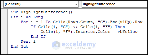
Code Breakdown:
- Dim i As Long → Declares a variable i to use as a loop counter.
- For i = 1 To Cells(Rows.Count, “C”).End(xlUp).Row
If Cells(i, “C”) <> Cells(i, “F”) Then
Cells(i, “F”).Interior.Color = vbYellow
End If
This Loop goes through rows in column C, starting from row 1 and going up to the last non-empty row. It checks if the value in the current row of column C is different from the value in the same row of column F. If values are different, it changes the background color of the cell in column F to yellow.
- Next i → Refers to move to the next iteration of the loop.
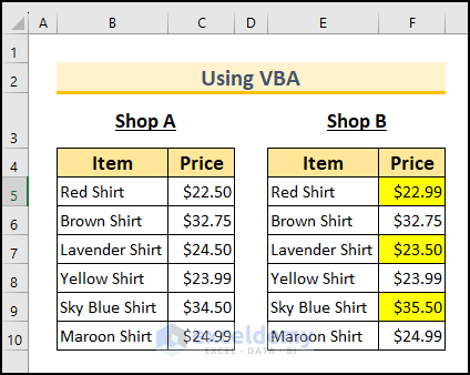
- Press F5 to run the code.
- The differences will be highlighted in the second table.
Method 3 – Apply Power Query to Compare Two Tables and Merge All Values
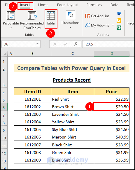
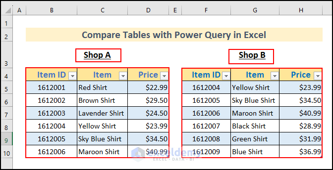
We have modified the dataset to illustrate this method. We have added a new column named Item ID to add more data to the dataset. We will convert all our dataset ranges into tables.
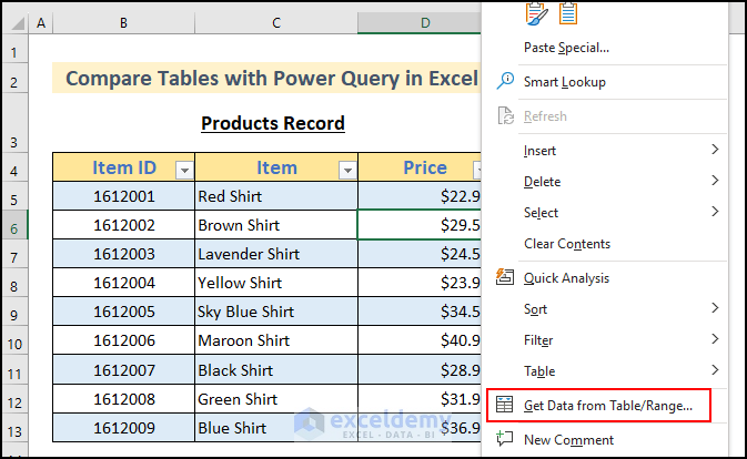
- Click on any cell of the Products Record range >> go to Insert tab >> Select Table.
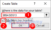
- From the Create Table window choose the range as B4:D13 >> tick on the option My table has headers >> click OK.
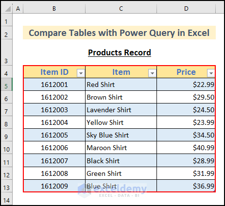
- The Products Record dataset will be converted into a table.
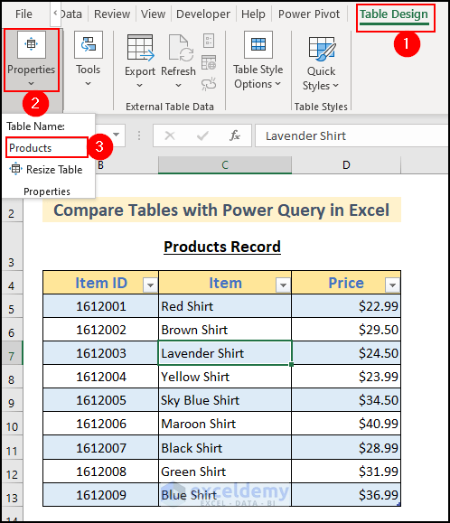
- To name this table, click on any value inside the table >> go to the Table Design tab >> Properties >> enter Products in the Table Name text box.
- Similarly, create two more tables named Shop_A and Shop_B from the individual Shop A and Shop B product records.
- Right-click on any cell inside the Products Record table and choose the Get Data from Table/Range option from the context menu.
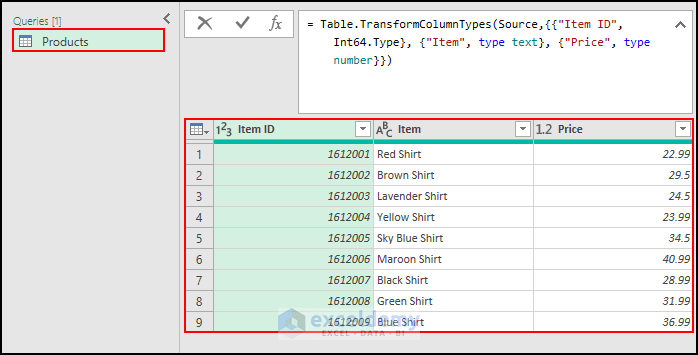
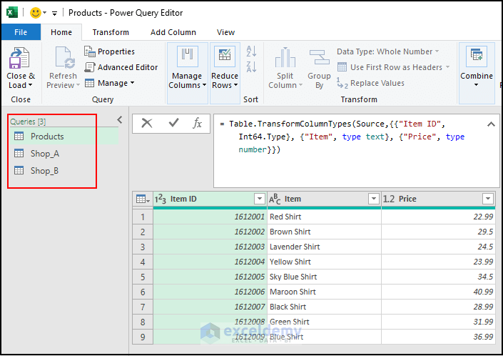
- You can see that the Products table is shown in the Power Query.
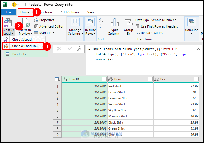
- In the Home tab of the Power Query, click on the arrow inside the Close & Load button >> choose the option Close & Load To.
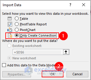
- Select the radio button on the option Only Create Connection and click OK from the Import Data box.
- Repeat the procedures individually for the Shop_A and Shop_B tables to import data from the given tables to Power Query.
- Right-click on the Queries pane area >> choose the New Query option >> Other Sources option >> Select Blank Query.
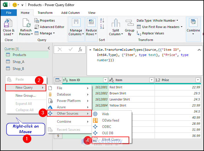
- A new query will be created.
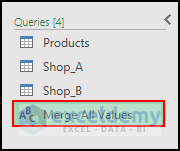
- Rename it as “Merge All Values”.
- Click on the Merge All Values query and enter the following formula to compare two tables and merge values through the power query.
- Press Enter.
=List.Union({Shop_A[Name],Shop_B[Name]},Comparer.OrdinalIgnoreCase)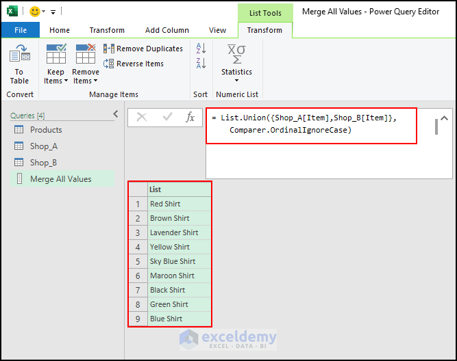
We have compared and merged two tables and got all the unique items from Shop A and Shop B.
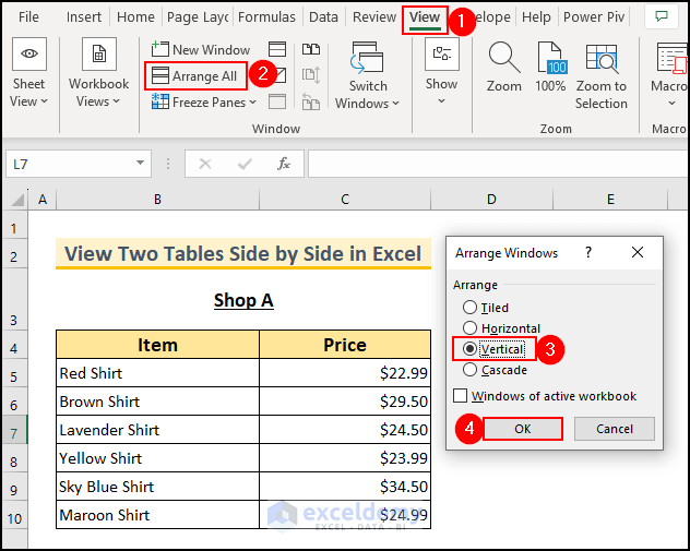
Method 4 – View Two Tables Side by Side in Excel to Compare Them
We can arrange two Excel windows side by side using “View Side by Side” mode. Using this method, we can visually compare two workbooks or two sheets in a single workbook.
- Open both Excel files you want to compare.
- Go to the View tab>> Window group>> Arrange All.
- Select Vertical from Arrange Windows and click OK.
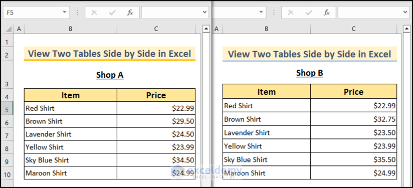
- The two Excel windows will appear side-by-side as shown in the following image.
Click the image for a detailed view
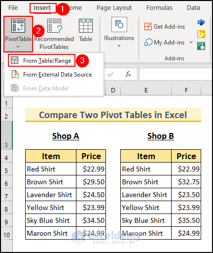
Method 5 – How Can You Compare Two Pivot Tables in Excel
Step 1 – Creating Two Pivot Tables in One Sheet
We will create two pivot tables in one sheet using the two datasets for Shop A and Shop B.
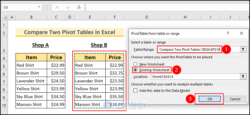
- Go to the Insert tab >> PivotTable drop-down >> Select From Table/Range.
- Select the range of the first table for Shop A in the Table/Range text box from the PivotTable from table or range dialog box.
- Select New Worksheet and click OK.
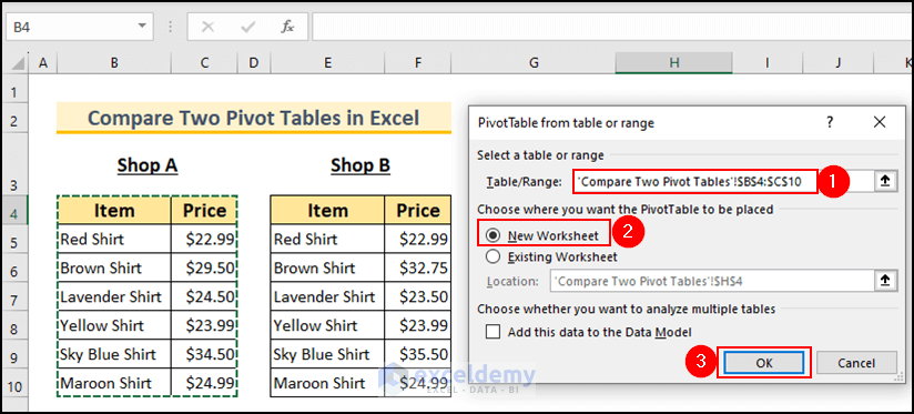
Click the image for a detailed view
- You’ll get a new sheet where you will have two portions; PivotTable1 and PivotTable Fields.
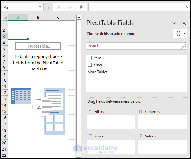
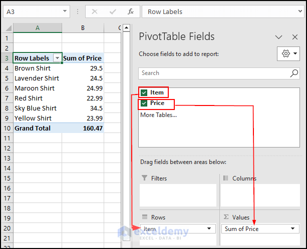
- Drag down Item to Rows area and Price to the Values.
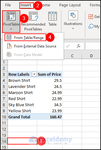
- To insert the second table in this same sheet, we have to insert the table again.
- Select cell A14 or any other cell where you want to enter the second PivotTable.
- Go to the Insert tab >> PivotTable dropdown >> Select From Table/Range.
- Select the range of the second table for Shop B in the Table/Range text box in the PivotTable from table or range dialog box.
- The Existing Worksheet option and the Location value will be selected automatically.
- Click OK.
Click the image for a detailed view
- Drag down Item to the Rows area and Price to the Values.
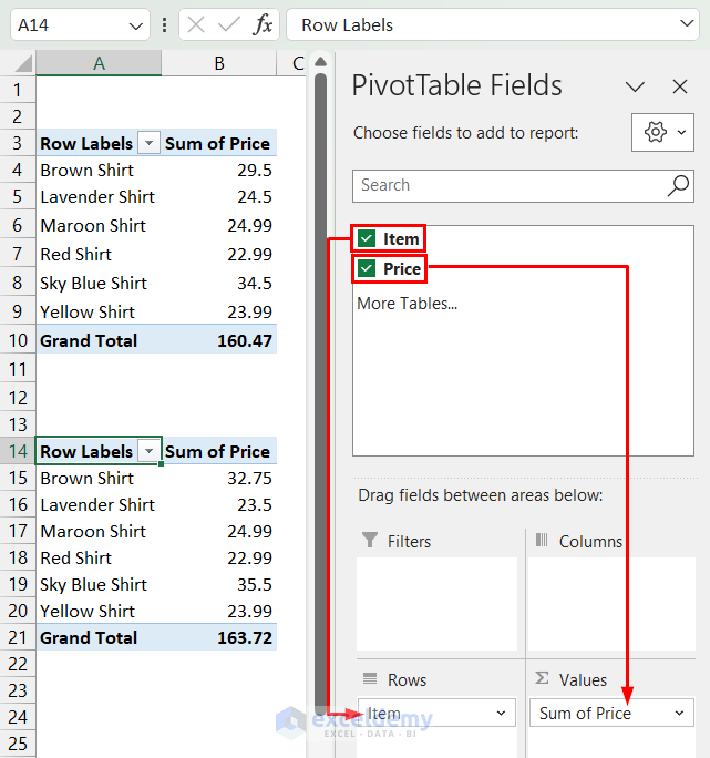
- We have inserted two pivot tables in one sheet.
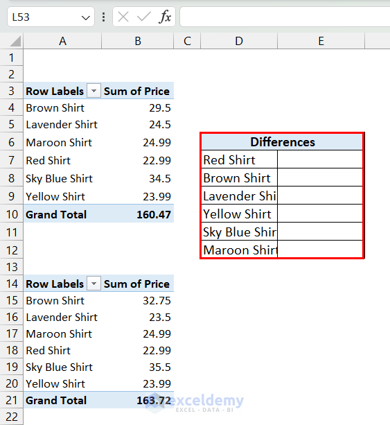
- We created a space for gathering the differences between different items following the second table.
Step 2 – Inserting the Formula to Calculate Differences Between Pivot Tables
- Enter the following formula in cell B26.
=GETPIVOTDATA("Sum of Price",$A$4,"Item",D8)-GETPIVOTDATA("Sum of Price",$A$15,"Item",D8)- Use the Fill Handle for the remaining cells.
- You will get the values for the rest of the cells and will be able to calculate all of the differences between the item prices for Shop A and Shop B.

Download Practice Workbook
Compare Tables in Excel: Knowledge Hub
<< Go Back to Compare | Learn Excel
Get FREE Advanced Excel Exercises with Solutions!
