Compare Two Tables and Highlight Differences in Excel (4 Methods)

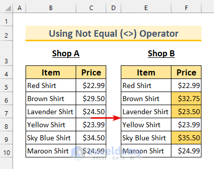
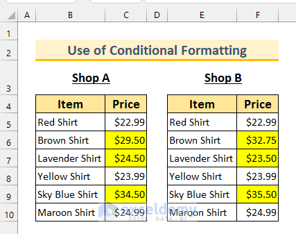
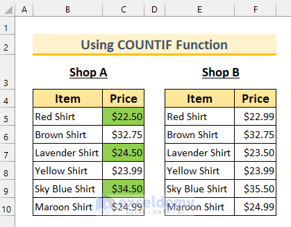
We have two tables that show the pricing of the same product in two shops. We’ll highlight the differences between the price columns.

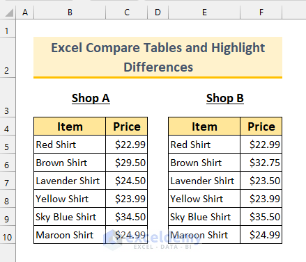
How to Compare Two Tables and Highlight Differences in Excel: 4 Ways

Method 1 – Using the Not Equal (<>) Operator with Conditional Formatting

Steps:

• Select the cell range F5:F10.
• From the Home tab, go to Conditional Formatting and select New Rule…

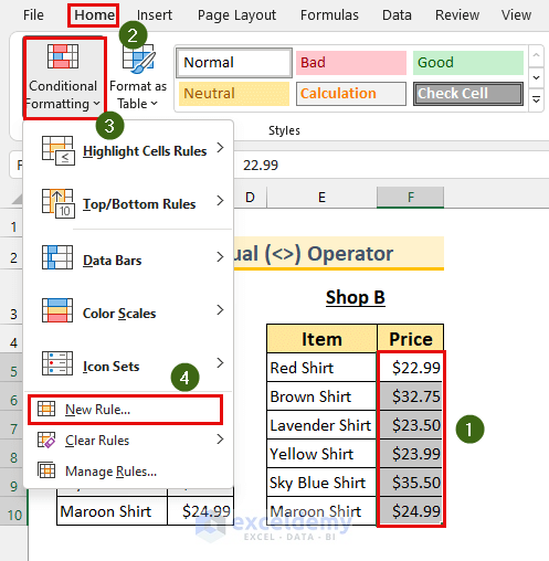
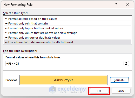
• The New Formatting Rule dialog box will appear.
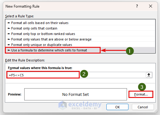
• Select Use a formula to determine which cells to format from the Select a Rule Type: section.
• Insert the following formula in the Edit the Rule Description: box.

We’re checking if the value from cell F5 is not equal to that of cell C5. If it is TRUE, then the cell will be highlighted.

• Click on Format…

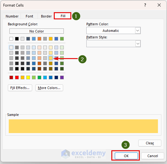
• The Format Cells dialog box will appear.
• Click on the Fill tab.
• Select a color from the Background Color: section.
• Press OK.

• Click on OK.

• Here are the results.

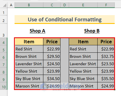
Method 2 – Using the Unique Conditional Formatting Rule

Steps:

• Select the full table cell range B4:F10.

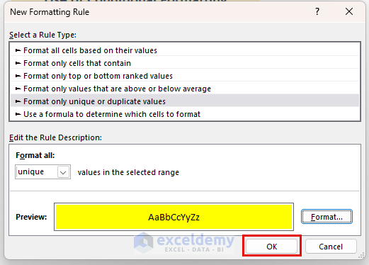
• Bring up the New Formatting Rule dialog box.
• Select Format only unique or duplicate values from the Rule Type section.
• Select unique from the Format all: box.
• Select a background color with the Format button.

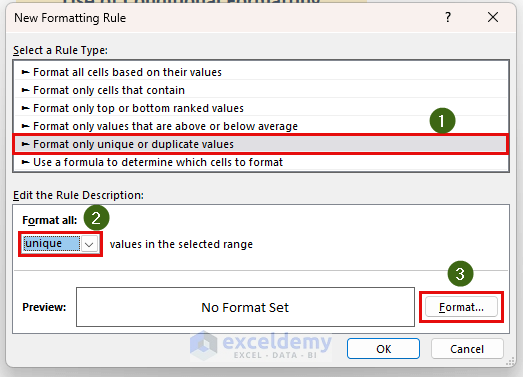
• Click on OK.

• This highlights all unique values between the tables. Note that if two different items happen to get the same price, they won’t be highlighted.

Method 3 – Implementing the COUNTIF Function to Compare Two Tables and Highlight the Differences in Excel

Steps:

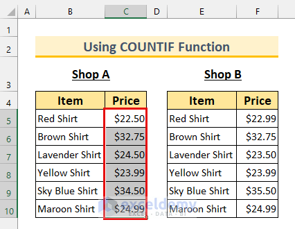
• Select the cell range C5:C10.
• Bring up the New Formatting Rule dialog box.

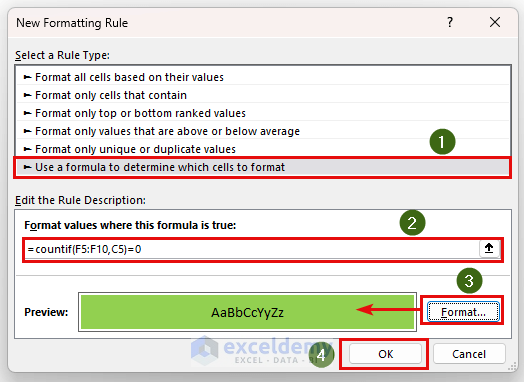
• Select Use a formula to determine which cells to format from the Select a Rule Type: section.
• Use the following formula in the Edit the Rule Description: box.

We’re checking if our value from the Column C is in the Column F. If it is not there, we’ll get 0. We’re formatting the cells which are not found in the F5:F10 cell range.

Note: This formula will only work for unique values. If your table has duplicate values (for example, two shirts have the same price), do not use this method.

• Pick a background color via the Format button.
• Press OK.

• Here’s the result.

Method 4 – Using VBA in Excel to Compare Two Tables and Highlight the Differences

Steps:

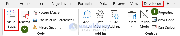
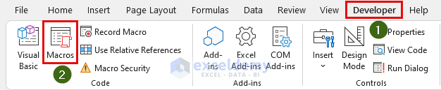
• From the Developer tab, select Visual Basic.
• This will bring up the Visual Basic window.

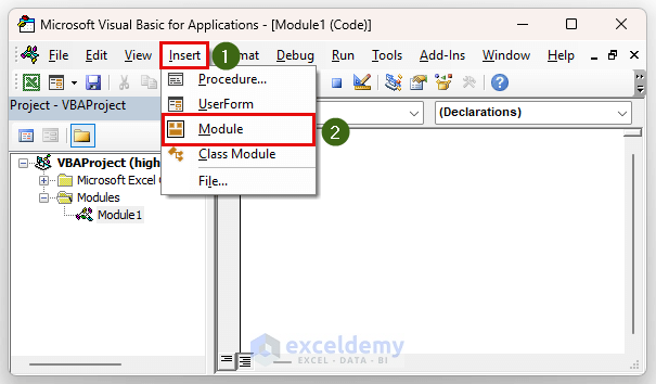
• From Insert, select Module.

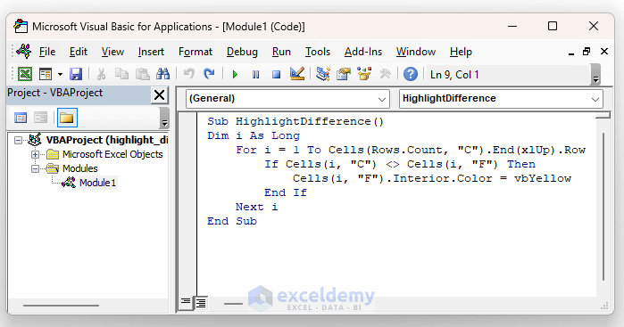
• Insert the following code in the module.

Sub HighlightDifference()
Dim i As Long
    For i = 1 To Cells(Rows.Count, "C").End(xlUp).Row
        If Cells(i, "C") <> Cells(i, "F") Then
            Cells(i, "F").Interior.Color = vbYellow
        End If
    Next i
End Sub

• Save the Module and close the window.
• From the Developer tab, select Macros.

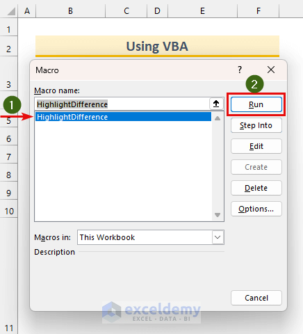
• The Macro dialog box will appear.
• Select HighlightDifference and click on Run.

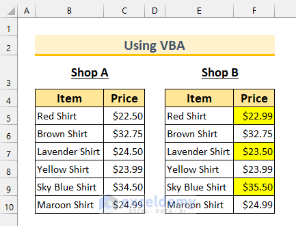
• You’ll see the differences highlighted in the second table.

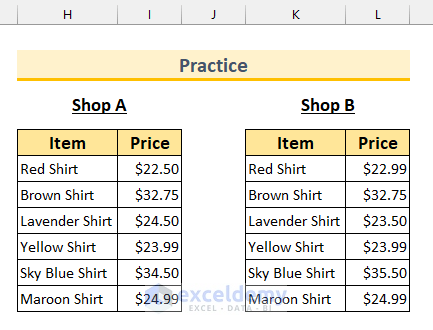
Practice Section

We’ve supplied practice datasets with each method in the Excel file.

Download the Practice Workbook

<< Go Back to Tables | Compare | Learn Excel