If we need to compare two tables in Excel, we can use the VLOOKUP function. It’s an easy way to compare two tables and find missing values, common values or return a value from a third column. Are you having trouble comparing two tables using the VLOOKUP function? This article will help you to learn how to compare two tables in Excel using the VLOOKUP function. Let’s get started!
How to Compare Two Tables in Excel Using VLOOKUP Function: 6 Ideal Examples
In this article, we will show you 6 ideal examples to compare two tables in Excel using the VLOOKUP function. It will help you compare two dataset columns in different scenarios. We will learn how to compare two columns in the same worksheet and how to compare two columns from different worksheets also.
1. Compare Two Columns in Same Worksheet
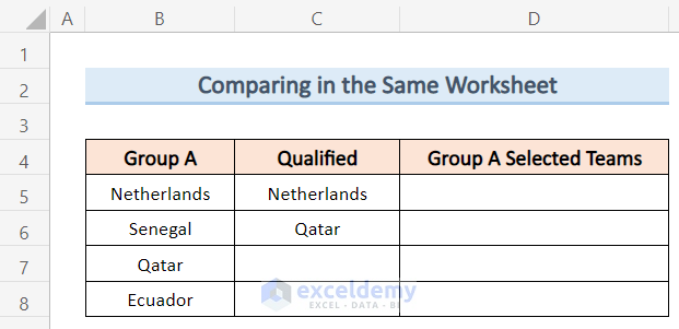
Comparing two columns in the same worksheet is the most common case in our daily life. It can be done easily using the VLOOKUP function. In order to demonstrate this example, we have taken a dataset like the following figure where we have 4 Teams from Group A and the Qualified teams from Group A. Now we will compare these two columns of tables in excel using the VLOOKUP function and display the common teams between the two columns in the column Group A Selected Teams.
In order to compare the two tables using the VLOOKUP function, follow the steps below.
Steps:
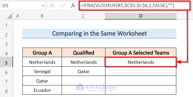
- First, select cell D5 and type the following formula:
=IFNA(VLOOKUP(B5,$C$5:$C$6,1,FALSE),"")- Second, press Enter and since Netherlands is a qualified team from Group A, you will see it in cell D5.
- Third, select the D5 cell and drag the Fill Handle to the entire column Group A Selected Teams.
- As a result, you will see an output like the image below where the common teams between the two columns will be displayed in column Group A Selected Teams.

🔎 How Does the Formula Work?
- VLOOKUP(B5,$C$5:$C$6,1,FALSE): Firstly, this part of the formula looks for B5 in the range ($C$5:$C$6). Then, returns the value from Column B. If the statement is False, it will display #N/A in the cell.
- IFNA(VLOOKUP(B5,$C$5:$C$6,1,FALSE),””): Finally, the IFNA function finally removes the #N/A if the statement was False and gives the final output.
2. Compare Two Columns in Different Worksheets
In order to compare two columns of tables in different excel worksheets using the VLOOKUP function, we have taken a dataset like the following figure where we have 4 Teams from Group A in sheet 1.

And we have the Qualified teams from Group A in sheet 2.
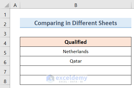
Now we will compare these two columns using the VLOOKUP function and display the common teams between the two columns in the column Group A Selected Teams in sheet 1. In order to compare two columns from different sheets using the VLOOKUP function, follow the steps below:
Steps:
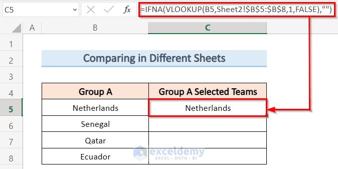
- Firstly, select cell C5 and type the following formula:
=IFNA(VLOOKUP(B5,Sheet2!$B$5:$B$8,1,FALSE),"")- Secondly, press Enter and since Netherlands is a qualified team from Group A, you will see it in cell C5.
- Thirdly, select the C5 cell and drag the Fill Handle to the entire column Group A Selected Teams.
- Finally, you will see an output like the image below where the common teams between the two columns will be displayed in column Group A Selected Teams.

🔎 How Does the Formula Work?
- VLOOKUP(B5,Sheet2!$B$5:$B$8,1,FALSE): Firstly, this part of the formula looks for B5 in the range (Sheet2!$B$5:$B$8). Then, returns the value from Column B. If the statement is False, it will display #N/A in the cell.
- IFNA(VLOOKUP(B5,Sheet2!$B$5:$B$8,1,FALSE),””): Finally, the IFNA function finally removes the #N/A if the statement was False and gives the final output.
3. Finding Common Values Between Two Columns
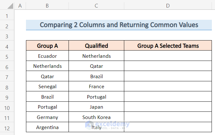
If we want to compare two columns of tables in the same Excel worksheet and find the common values between them, it can be done easily using the VLOOKUP function. In order to solve this example, we have taken a dataset like the following figure where we have 8 Teams from Group A and the 8 Qualified teams in total. Now we will compare these two columns using the VLOOKUP function and display the teams qualified from Group A.
Follow the steps below in order to compare two columns and find missing values using the VLOOKUP function.
Steps:
- First of all, select cell D5 and type the following formula:
=FILTER(B5:B12, IFNA(VLOOKUP(B5:B12, C5:C12, 1, FALSE), "")<>"")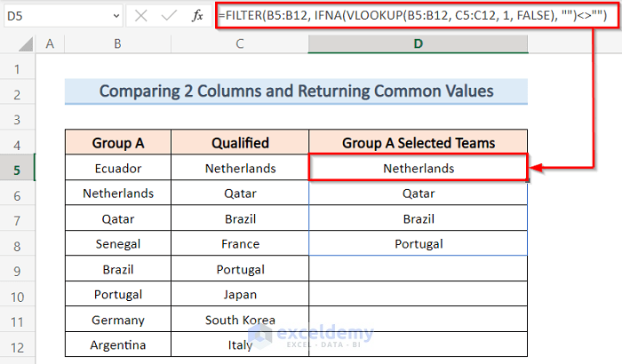
- Second, press Enter and since it is an array formula, you will see all the selected teams from Group A under the column Group A Selected Teams like the image below.

🔎 How Does the Formula Work?
- VLOOKUP(B5:B12, C5:C12, 1, FALSE): Firstly, this part of the formula looks for (B5:B12) in the range (C5:C12).
- IFNA(VLOOKUP(B5:B12, C5:C12, 1, FALSE): Secondly, the IFNA function finds if the statement is True.
- FILTER(B5:B12, IFNA(VLOOKUP(B5:B12, C5:C12, 1, FALSE), “”)<>””): Finally, the FILTER function sorts all the TRUE statements and give the final output.
4. Finding Missing Values Between Two Columns
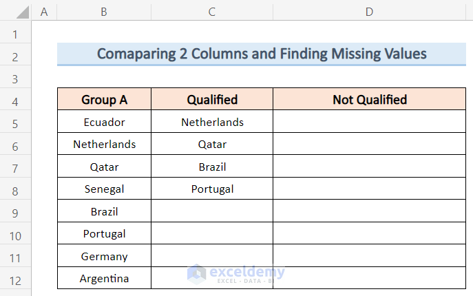
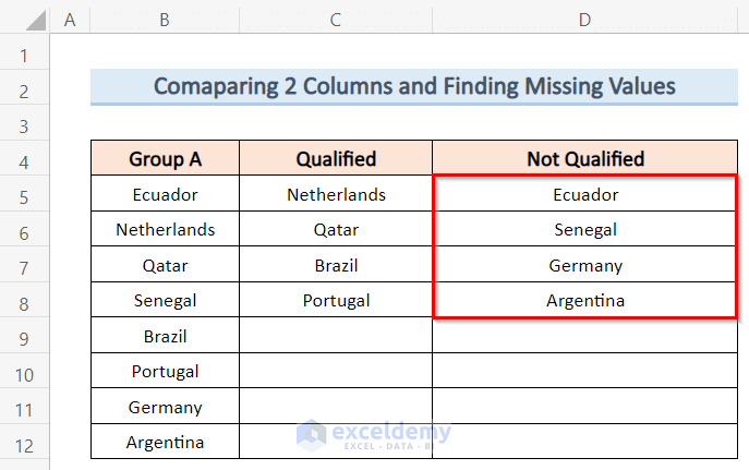
If we want to compare two columns and find the difference between them, it can be done easily using the VLOOKUP function. In order to solve this example, we have taken the same dataset as the following figure where we have 8 Teams from Group A and 4 Qualified teams from Group A. Now we will compare these two columns of tables using the Excel VLOOKUP function and display the Not Qualified teams from Group A.
Follow the steps below in order to compare two columns and find missing values using the VLOOKUP function.
Steps:
- To begin with, select cell D5 and type the following formula:
=FILTER(B5:B12,ISNA(VLOOKUP(B5:B12,C5:C8,1,FALSE)))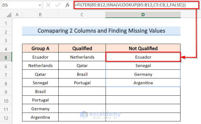
- Lastly, press Enter and since it is an array formula, you will see all the Not Qualified teams from Group A under the column Not Qualified like the image below.
🔎 How Does the Formula Work?
- VLOOKUP(B5:B12,C5:C8,1,FALSE): Firstly, this part of the formula looks for B5:B12 in the range (C5:C8).
- ISNA(VLOOKUP(B5:B12,C5:C8,1,FALSE)): Secondly, the ISNA function finds all the statements which are False.
- FILTER(B5:B12,ISNA(VLOOKUP(B5:B12,C5:C8,1,FALSE))): Finally, the FILTER function function sorts all the FALSE statements and give the final output.
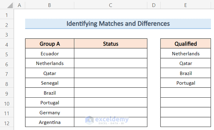
5. Identifying Matches and Differences Between Two Columns
Now to identify matches and differences between 2 columns using the VLOOKUP function, we have taken a dataset like the following figure where we have 8 Teams from Group A and 4 Qualified teams from Group A in another column. Now we will compare these two columns using the VLOOKUP function and find matches and differences. After finding the matches and differences, we will insert the status either Qualified or Not Qualified in the Status column.
In order to compare two columns using the VLOOKUP function, follow the steps below:
Steps:
- Firstly, select cell C5 and type the following formula:
=IF(ISNA(VLOOKUP(B5,$E$5:$E$8,1,FALSE)),"Not Qualified","Qualified")- Secondly, press Enter and since Ecuador is not a qualified team from Group A, you will see Not Qualified status for this team.
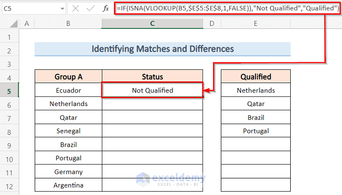
- Thirdly, select the C5 cell and drag the Fill Handle to the entire column Status.
- Finally, you will see an output like the image below where the qualified teams will have the status Qualified and the not qualified teams will have the status Not Qualified.

🔎 How Does the Formula Work?
- VLOOKUP(B5,$E$5:$E$8,1,FALSE): Firstly, this part of the formula looks for B5 in the range ($E$5:$E$8).
- ISNA(VLOOKUP(B5,$E$5:$E$8,1,FALSE)): Secondly, the ISNA function finds all the statements which are False.
- IF(ISNA(VLOOKUP(B5,$E$5:$E$8,1,FALSE)),”Not Qualified”,”Qualified”): Finally, the IF function gives the output Qualified if it is a match and gives output Not Qualified if it does not match.
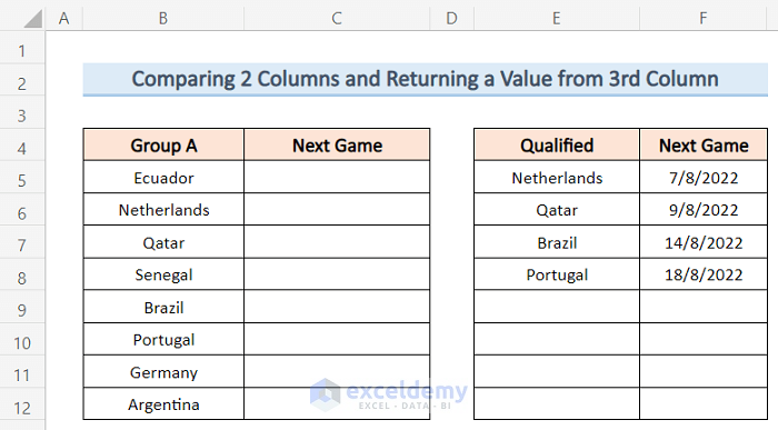
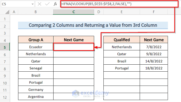
6. Compare Two Columns and Return a Value from 3rd Column
Sometimes we have to return a value from the third column in Excel. In order to compare two columns and return a value from 3rd column using the VLOOKUP function, we have taken a dataset like the following figure where we have 8 Teams from Group A and 4 Qualified teams from Group A and their Next Game date in Columns E and F. Now we will compare these two columns using the VLOOKUP function and return the Next Game date for the qualified teams in Column C.
To compare two columns using the VLOOKUP function and return a value from 3rd column, follow the steps below:
Steps:
- First, select cell C5 and type the following formula:
=IFNA(VLOOKUP(B5,$E$5:$F$8,2,FALSE),"")- Second, press Enter and since Ecuador is not a qualified team from Group A, you will see a blank space for this team.
- Third, select the C5 cell and drag the Fill Handle to the entire column Next Game.
- Finally, you will see an output like the image below where the qualified teams will have the Next Game date and the not qualified teams will have blank spaces in the column Next Game.

🔎 How Does the Formula Work?
- VLOOKUP(B5,$E$5:$F$8,2,FALSE): Firstly, this part of the formula looks for B5 in the range ($E$5:$F$8).
- IFNA(VLOOKUP(B5,$E$5:$F$8,2,FALSE),””): Finally, the IFNA function finds if the statement is True and gives the output when the statement is True.
Things to Remember
- The FILTER function is only available in Microsoft Office 365. So if you have an older version of Microsoft Office, you won’t be able to use this function.
- You don’t need to use Fill Handle for the FILTER function. Since it is an array formula, it will automatically sort all the values and give you the output.
Download Practice Workbook
You can download the Excel workbook from here.
Conclusion
Hence, follow the above-described steps. Thus, you can easily learn how to compare two tables in Excel VLOOKUP. Hope this will be helpful. Don’t forget to drop your comments, suggestions, or queries in the comment section below.
<< Go Back to Tables | Compare | Learn Excel


Dear Asaduzzaman,
Your post has been for a great help for me. Much appreciated
Keep it up
Hello, Andre!
Thanks for your appreciation. To get more helpful posts stay in touch with ExcelDemy.
Regards
ExcelDemy