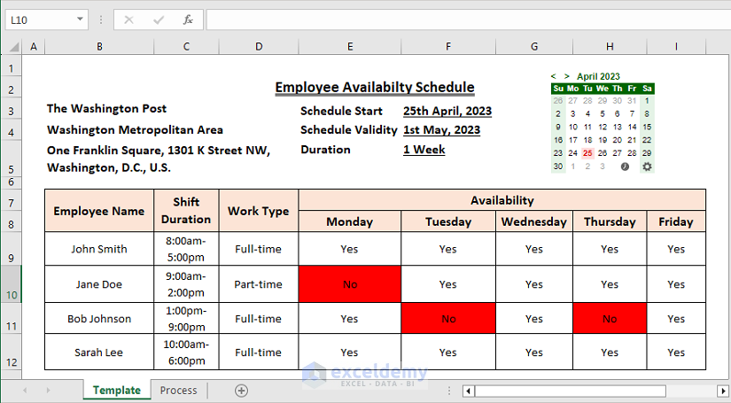
How to Make an Availability Schedule in Excel (with Easy Steps)

In this article, we’ll demonstrate how to create an availability schedule template in Excel, as in the video and image below.

Watch Video – Make an Availability Schedule in Excel

How to Make an Availability Schedule Template in Excel: Step-by-step Procedures

Use the free template included at the download link at the bottom of this article, or follow the steps to make a similar type of template according to your needs.

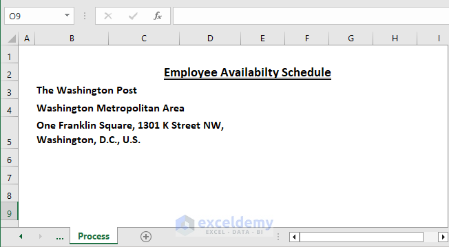
Step 1 – Add Necessary Header Information

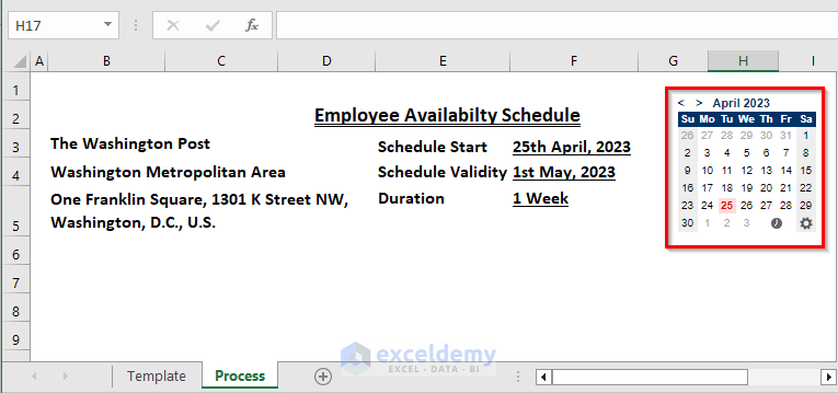
To begin with, for presentation purposes, add some header information such as the Scheduling table title, Company name, Jurisdiction area and Office location.

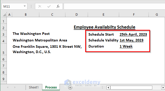
Step 2 – Add a Validation Period to Your Availability Scheduling

Add the Schedule start date from which this schedule will be applicable along with the date when this schedule will expire. You can also mention the duration of this schedule.

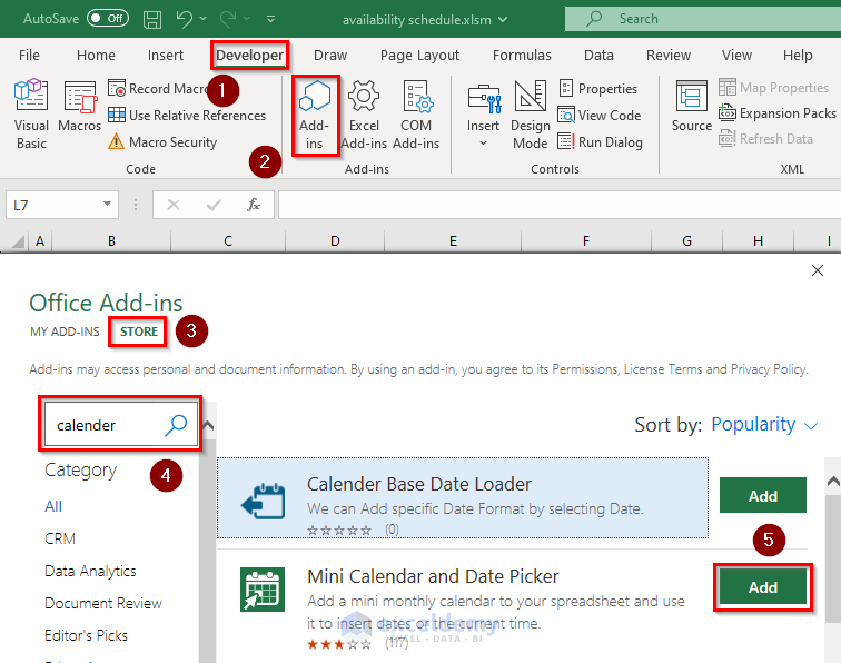
Step 3 – Add a Calendar to Match Weekly Days and Dates Easily

Optionally, add a display calendar.

Click on Add-ins under the Developer tab.
Inside the window that pops up, click on STORE.
Inside the search bar type “calendar” and press ENTER.
From the search result, click on the Add button beside Mini Calendar and Date Picker.

A mini calendar will be visible on your worksheet. Resize and place it anywhere suitable.

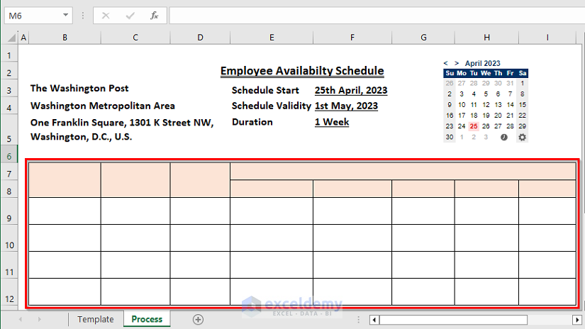
Step 4 – Build a Skeleton of Your Availability Scheduling Table

Now create a table to accommodate your scheduling information.

Specify the number of rows and columns and draw the table accordingly.
Optionally, merge cells inside any rows or columns to give the table a more organized and suitable look.

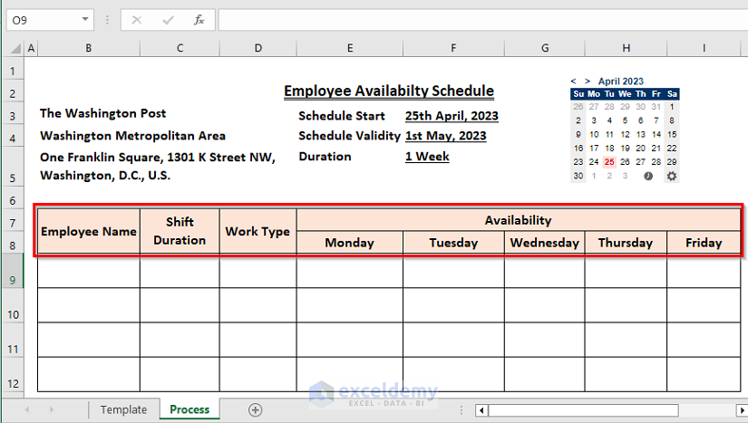
Step 5 – Add Necessary Headings to Each Column

After building the table skeleton, provide the necessary headings to the columns just added to the table. Add as many columns as needed to accommodate necessary information inside the table, but avoid unnecessary columns which might damage the integrity of the table.

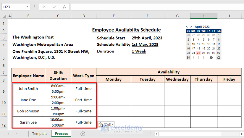
Step 6 – Add Necessary Data to Each of the Rows

The number of rows is equal to the number of people for whom the scheduling is applicable. Add as many people as needed and fill the rows with corresponding information according to the columns.

Step 7 – Generate a VBA Worksheet Event to Improve Readability

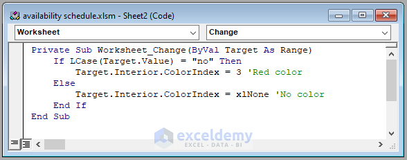
Finally, we can generate the following VBA code which will automatically turn the cell color red whenever an employee is not available for any particular day. If that person is in fact available, the cell will revert to colorless automatically.

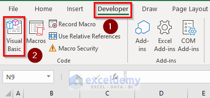
If you are using VBA for the first time, you may need to add the Developer tab to the main Excel ribbon.

To enter the VBA Code:

Launch the Visual Basic Editor by clicking on Visual Basic under the Developer tab.

Double-click on the sheet name in which to apply the code.

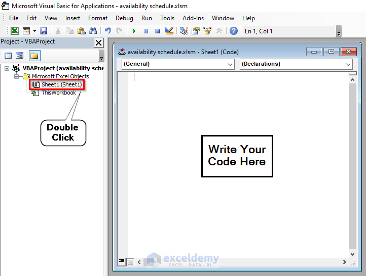
Inside the worksheet event, enter the code below.

Code Syntax:

Private Sub Worksheet_Change(ByVal Target As Range)
If LCase(Target.Value) = "no" Then
Target.Interior.ColorIndex = 3 'Red color
Else
Target.Interior.ColorIndex = xlNone 'No color
End If
End Sub

Code Breakdown:

Private Sub Worksheet_Change(ByVal Target As Range)

Defines a worksheet event procedure that runs whenever a cell on the worksheet is changed.

If LCase(Target.Value) = "no" Then

Uses the LCase function to convert the value in the target cell to lowercase, and checks if it is equal to “no“.

Interior.ColorIndex = 3 'Red color

If the value in the target cell is “no“, the cell interior color is set to red.

Else

If the value in the target cell is not “no“, begins the Else block.

Interior.ColorIndex = xlNone 'No color

Sets the cell interior color to no color (the default color) if the value in the target cell is not “no“.

End If

Ends the If statement.

End Sub

Ends the worksheet event procedure.

To activate this code, type “No” inside the corresponding cell where the employee is unavailable. The cell will automatically turn red. If that employee is somehow available later, just replace the “No” with “Yes” and the cell will return to its colorless condition.

The code is written in such a way that whether you type “NO”, “No”, “nO” or “no”, it will convert the letters into lowercase, recognize them, and color the cell.

Things to Remember

Determine the purpose of the schedule and what information needs to be included in it. This will help you decide on the structure and layout of the schedule.
Make sure to include all important details in the schedule, such as shift duration, work type, employee name, and date. This will ensure that the schedule is accurate and useful.

Download Practice Workbook

How to Make an Availability Schedule.xlsx