How to Create a Workback Schedule in Excel (with Easy Steps)

A Workback schedule is a vital element of our professional life. It helps us to track our tasks of running projects sequentially. In this article, we will demonstrate to you the step-by-step procedure to create a workback schedule in Excel. If you are also curious about it, download our practice workbook and follow us.

Watch Video – Create a Workback Schedule in Excel

What Is Workback Schedule?

Workback schedules show the timeline of a project in reverse order, starting with the delivery date and ending with the start date. When the only requirement is the due date of a project, reverse engineering the schedule is a good idea. When you have many moving parts in a complex project, a workback schedule is a useful tool to ensure that each task receives the attention it requires in a timely manner. The four major advantages of a workback schedule are:

It helps us to allocate our resources effectively.
Helps with proper time management.
Provide us with information on unrealistic task completion dates.
It helps us to create milestones.

How to Create a Workback Schedule in Excel: Step-by-Step Procedure

In this article, we will show you the step-by-step procedure to design a workback schedule in Excel.

📚 Note:

All the operations of this article are accomplished by using the Microsoft 365 application.

Step 1: Create Preliminary Summary Layout

In the first step, we will create the preliminary summary layout of the workback schedule report.

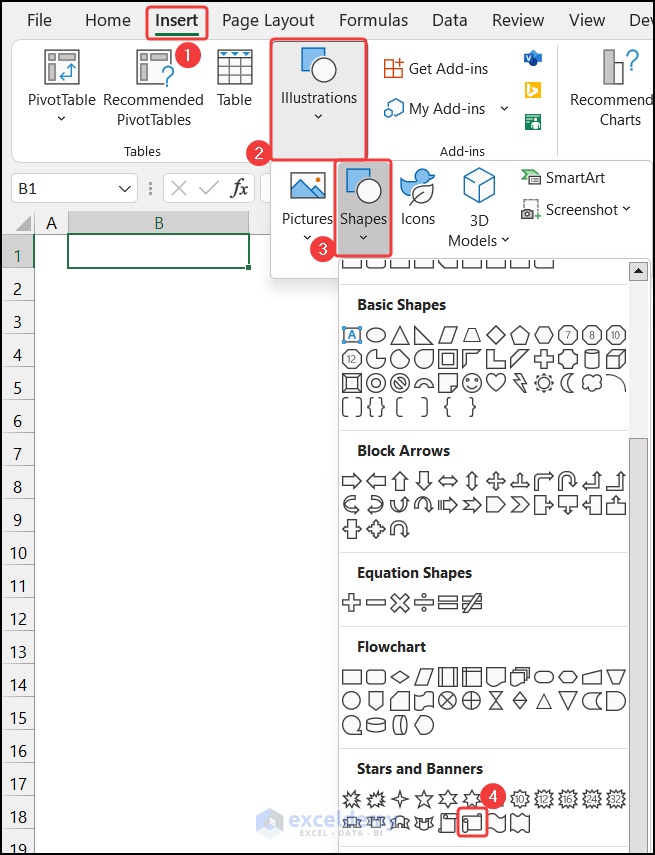
First of all, select cell B1.
Now, in the Insert tab, click on the drop-down arrow of the Illustration > Shapes option and choose a shape according to your desire. Here, we choose the Scroll: Horizontal shape.

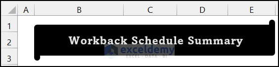
Then, write down the title of our report. In our case, we wrote Workback Schedule Summary as the sheet title.

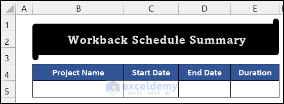
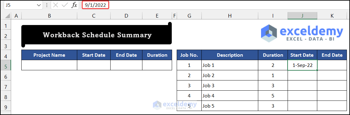
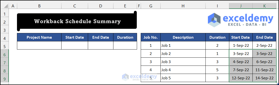
In the range of cells B4:E4, write down the following heading and allocate the corresponding range of cells B5:E5 to input the results.

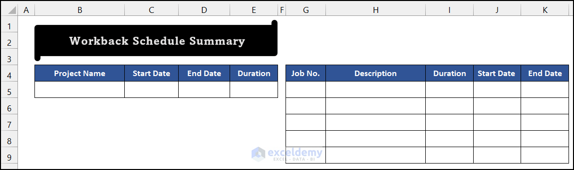
After that, in the range of cells G4:K4, write down the following entities to enlist the work plan.

Finally, select cell K1, and in the Insert tab, click on the drop-down arrow of the Illustration > Pictures option and choose the This Device command.

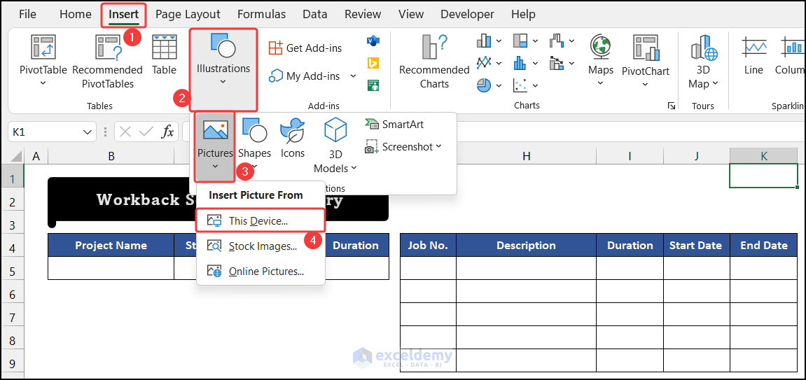
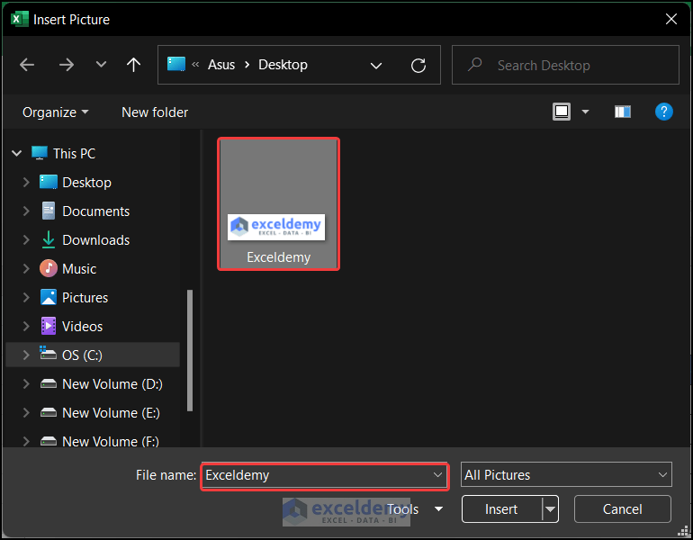
As a result, a small dialog box called Insert Picture will appear.
Afterward, choose your company logo. We chose our website logo to demonstrate the process.
Next, click on Insert.

Our job is completed.

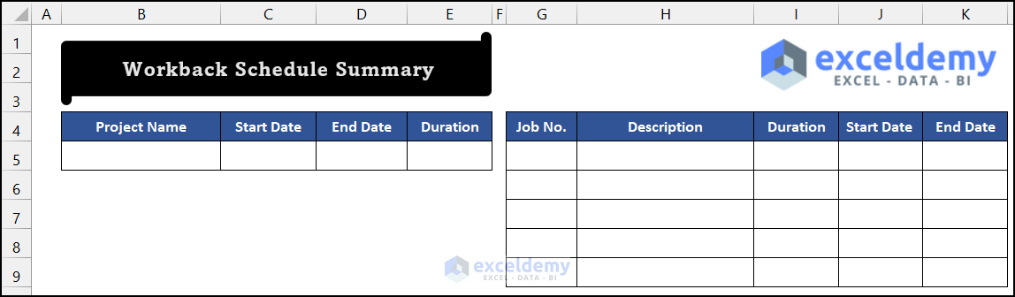
Thus, we can say that we have finished the first step, to create a workback schedule in Excel.

Step 2: Input Sample Dataset

In this step, we will input some sample data to check the accuracy of our formula and make our job easy.

First, in the range of cells G5:I5, input the following data.

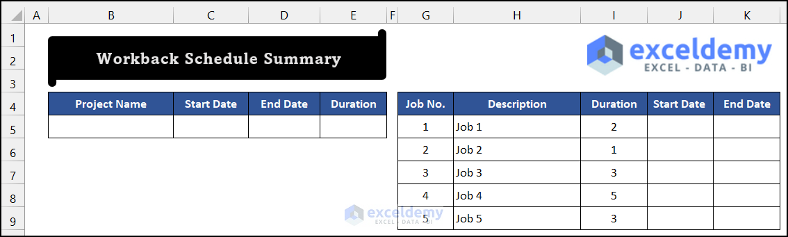
After that, in cell J5, write down the work starting date. We input 1-Sep-22.

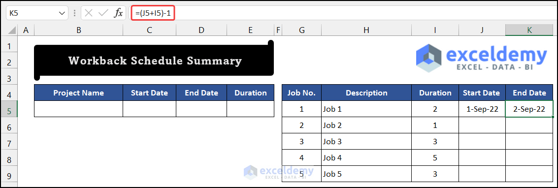
Now, to get the value of the End Date, write down the following formula in cell K5.

=(J5+I5)-1

Press Enter.

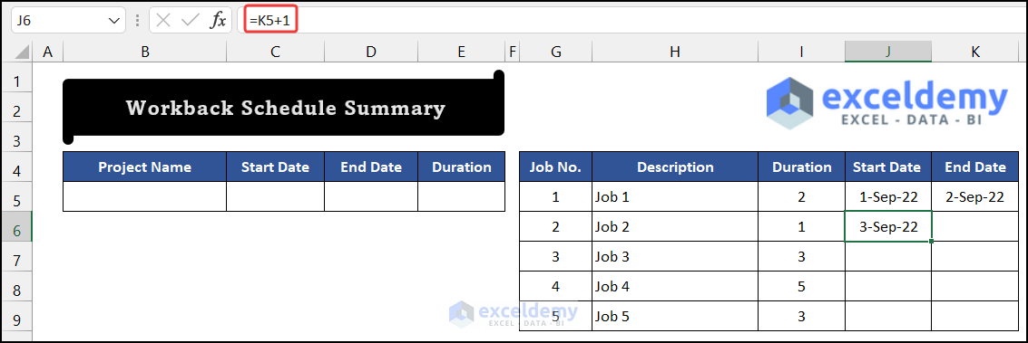
Then, the second task will start after finishing the first task. So, to get the starting date of the second task, write down the following formula.

=K5+1

Similarly, press Enter.

Afterward, select cell K5 and drag the Fill Handle icon to get the end date of Job 2.

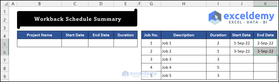
Next, select the range of cells I6:K6 and drag the Fill Handle icon to the last of your job list. We have 5 jobs. Hence, we dragged the Fill Handle icon up to cell K9.

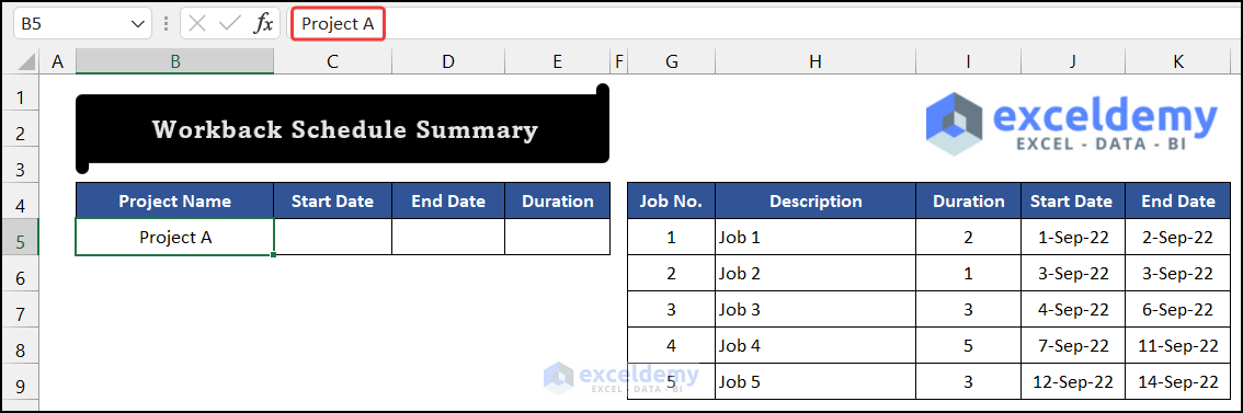
Now, select cell B5 and write down the Project Name.

Then, to get the Start Date of the project, select cell C5 and write down the following formula in the cell. For that, we will use the MIN function.

=MIN(J:J)

Again, press Enter.

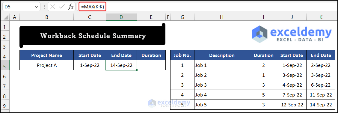
After that, for the End Date, write down the following formula in cell D5 using the MAX function.

=MAX(K:K)

Press Enter.

Finally, to get the Duration value of the project, write down the following formula in cell E5.

=(D5-C5)+1

Press Enter for the last time.

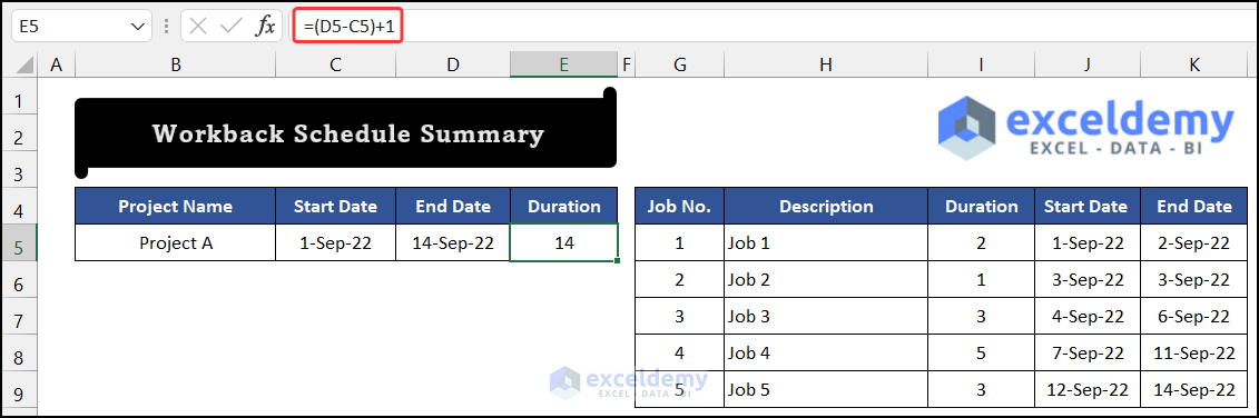
Our task is completed.

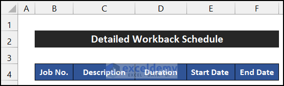
Therefore, we can say that we have completed the second step, to create a workback schedule in Excel.

Step 3: Import Dataset into Detail Workback Report

Now, we will import the job list from the Summary sheet to the Workback sheet.

First, write down the title of this sheet.
Then, write down the headings according to the last sheet.

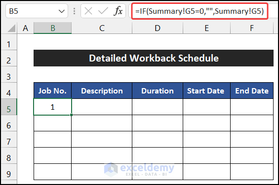
After that, to get the first job no., write down the following formula in cell B6, using the IF function.

=IF(Summary!G5=0,"",Summary!G5)

Press Enter.

Now, drag the Fill Handle icon to your right to get all other four entities up to cell F5.

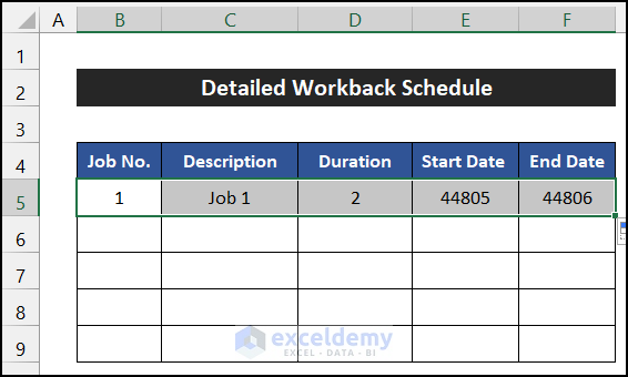
Then, select the range of cells B5:F5, and drag the Fill Handle icon to copy the formula up to cell F9.

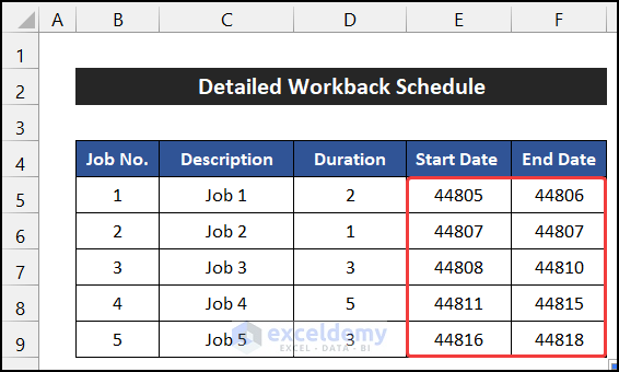
You may notice that the Start Date and End Date columns are showing some random number instead of the dates.

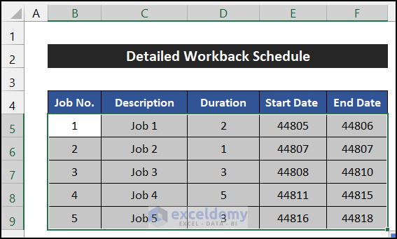
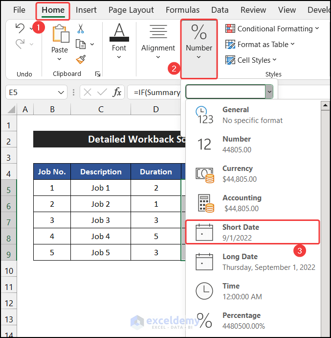
To fix this issue, select the range of cells E5:F9, and from the Number group, choose the Short Date formatting located in the Home tab.

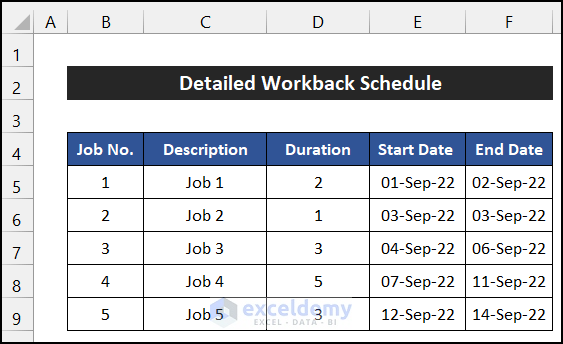
Our data importing task is finished.

Hence, we can say that we have accomplished the third step, to create a workback schedule in Excel.

Step 4: Creating Workback Gantt Chart

In the following step, we are going to create the Workback Gantt chart to visualize the work schedule more properly.

Firstly, we have to write down the dates of the corresponding month.
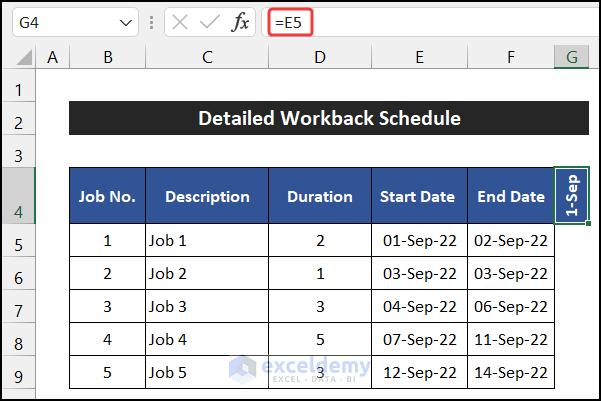
The first day of the project will be the first date of the Gantt chart. So, to get the date, select cell G4 and write down the following formula into the cell.

=E5

Press Enter.

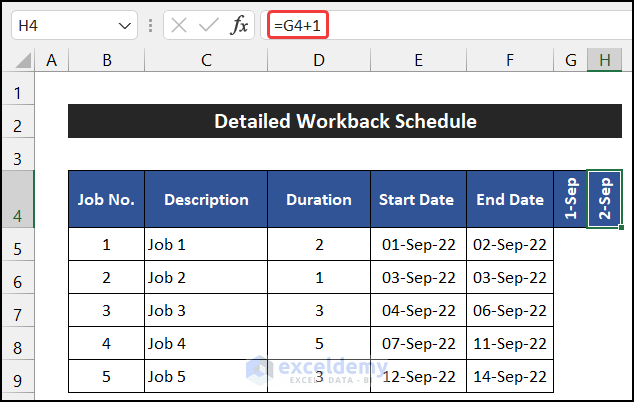
After that, select cell H4 and write down the following formula to get the next date.

=G4+1

Similarly, press Enter.

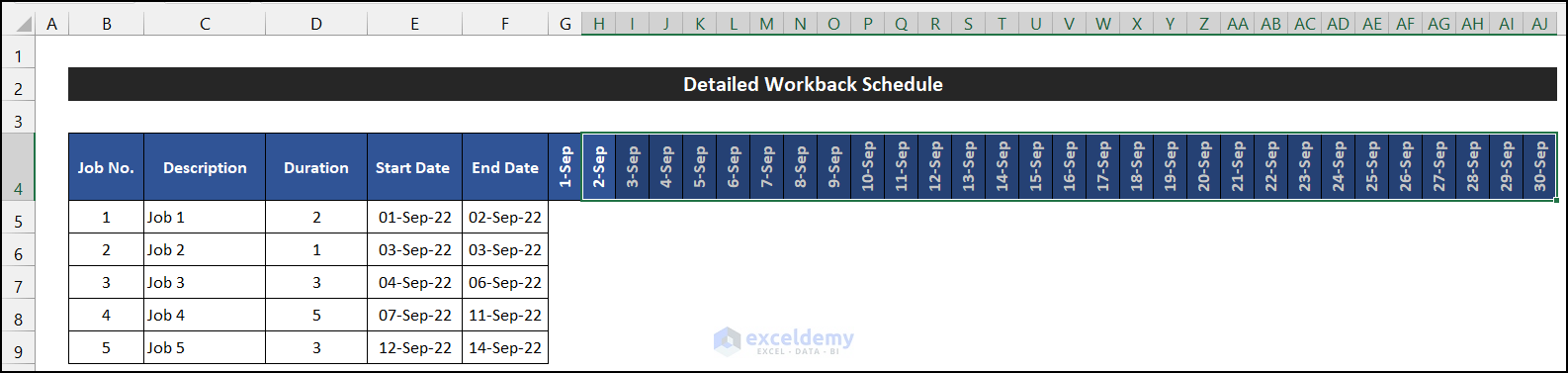
Now, select the H5 and drag the Fill Handle icon to get all the dates of that month up to cell AJ4.

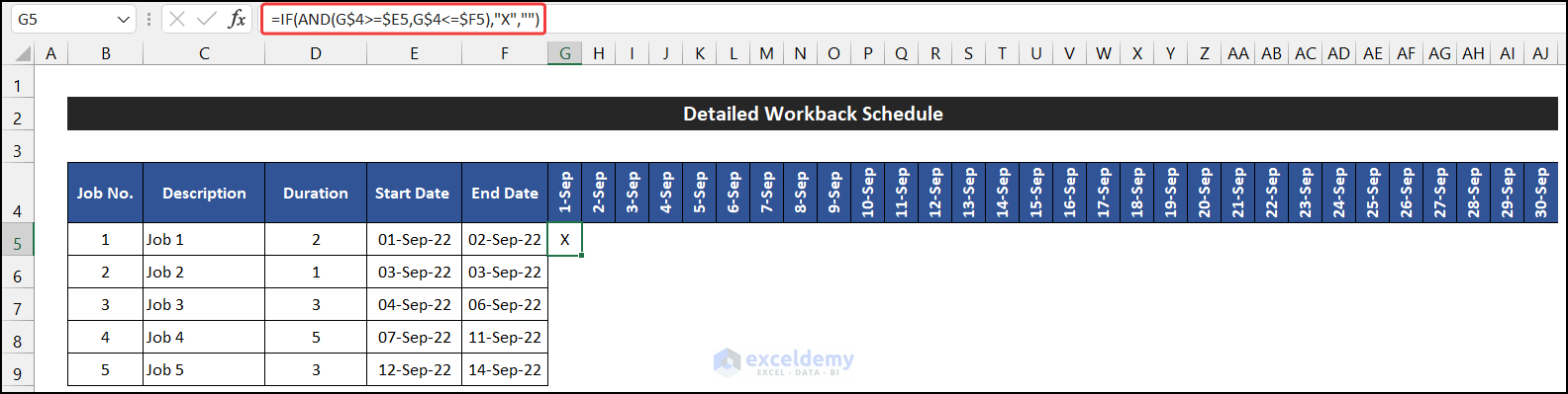
Then, select cell G5 and write down the following formula using the IF and AND functions.

=IF(AND(G$4>=$E5,G$4<=$F5),"X","")

🔎 Breakdown of the Formula

We are breaking down the formula for cell G5.

👉 AND(G$4>=$E5,G$4<=$F5): The AND function will check both logics. If both logics are true, the function will return TURE. Otherwise, it will return FALSE. For this cell, the function will return TRUE.

👉 IF(AND(G$4>=$E5,G$4<=$F5),”X”,””): The IF function will check the result of the AND function. If the result of the AND function is true, the IF function returns “X”. On the other hand, the IF function will return a blank.

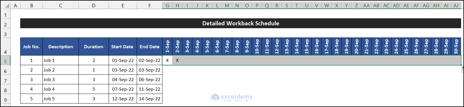
Again, press Enter.

Next, drag the Fill Handle icon to your right up to cell AJ6.

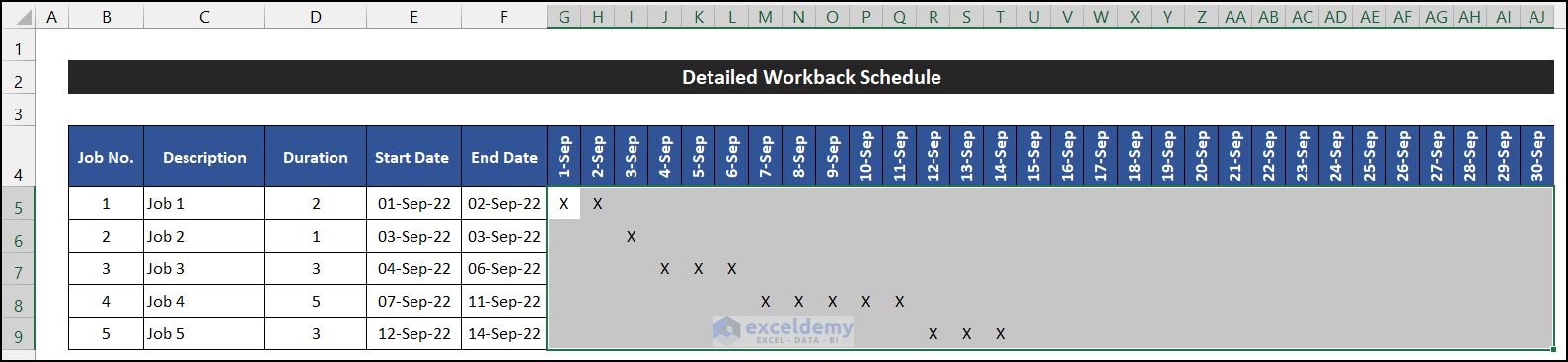
Afterward, select the range of cell G5:AJ5 and drag the Fill Handle icon to copy the formula up to AJ9.
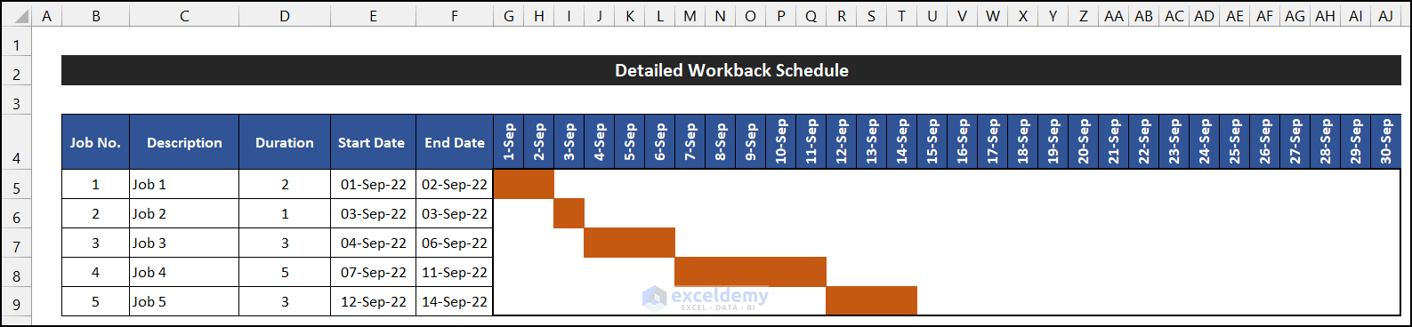
You will see all the dates along the job show the value X.

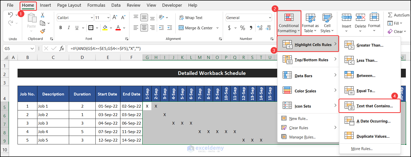
Now, in the Home tab, click on the drop-down arrow of the Conditional Formatting > Highlight Cell Rules option from the Style group and choose the Text that Contains command.

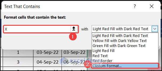
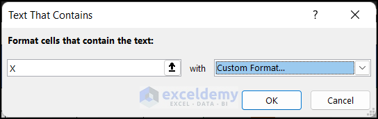
As a result, the Text That Contains dialog box will appear.
Write down X in the empty field, and in the next empty field, select the Custom Format option.

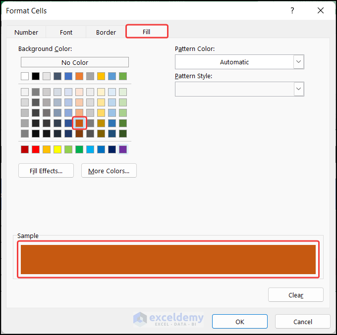
Another dialog box called the Format Cell will appear.
Then, in the Fill tab, choose the Orange, Accent 2, Darker 25% color.
Finally, click OK.

Again, click OK to close the Text That Contains dialog box.

At last, modify the text color with the same cell color.

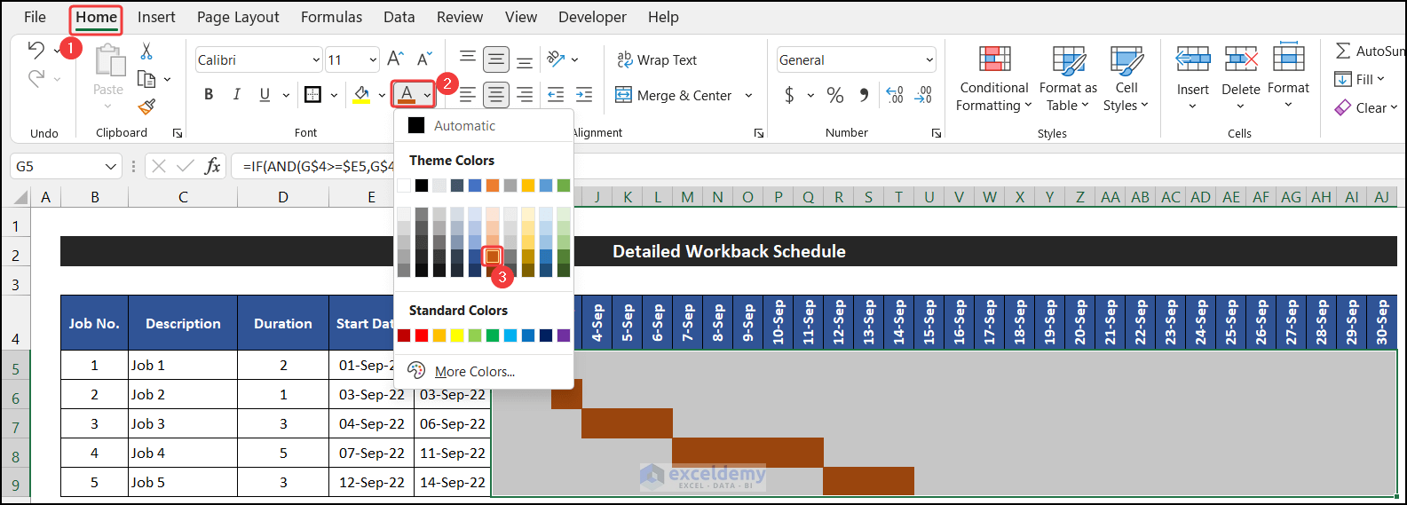
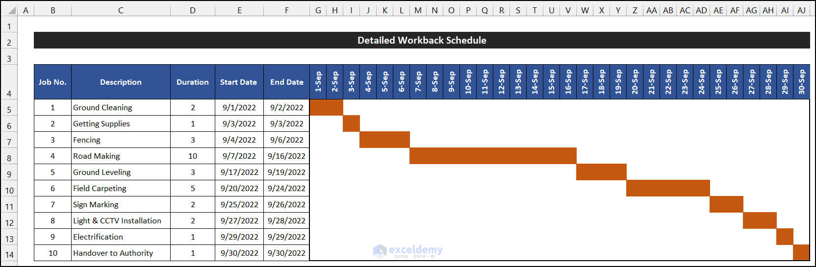
Our workback schedule is completed.

So, we can say that we have finished the final step, to create a workback schedule in Excel.

Step 5: Verify with New Dataset

In the final step, we will input another sample set of data to check our workback schedule report.

For that, in the Summary sheet, input a new dataset like the image shown below:

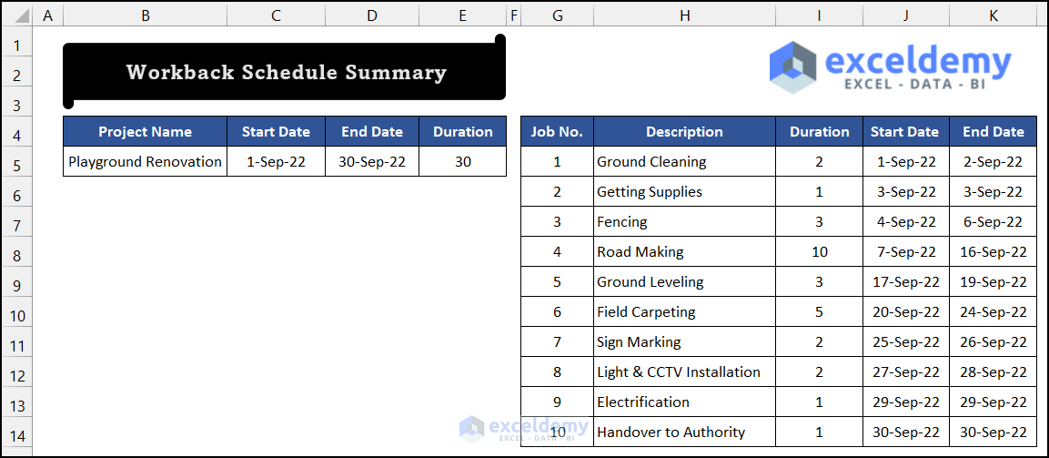
Now, go to the Workback sheet, and you will see the workback schedule will be updated.

Finally, we can say that all of our formulas and working procedures work successfully, and we are able to create a workback schedule in Excel.

Download Practice Workbook

Download this practice workbook for practice while you are reading this article.

Create a Workback Schedule.xlsx

Conclusion

That’s the end of this article. I hope that this article will be helpful for you and you will be able to create a Workback schedule in Excel. Please share any further queries or recommendations with us in the comments section below if you have any further questions or recommendations.

<< Go Back to Make Schedule in Excel | Excel for Business | Learn Excel

Get FREE Advanced Excel Exercises with Solutions!