How to Create a Monthly Schedule in Excel (3 Simple Ways)

Written by Arin Islam

Last updated: Jul 4, 2024

Watch Video – Create a Monthly Schedule in Excel

Method 1 – Using Excel Templates to Create Monthly Schedule in Excel

Step 1 – Inserting Excel Template

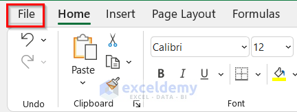
Click on the File tab.

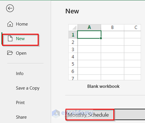
Go to New.
Type Monthly Schedule in the Search.
Click ENTER.

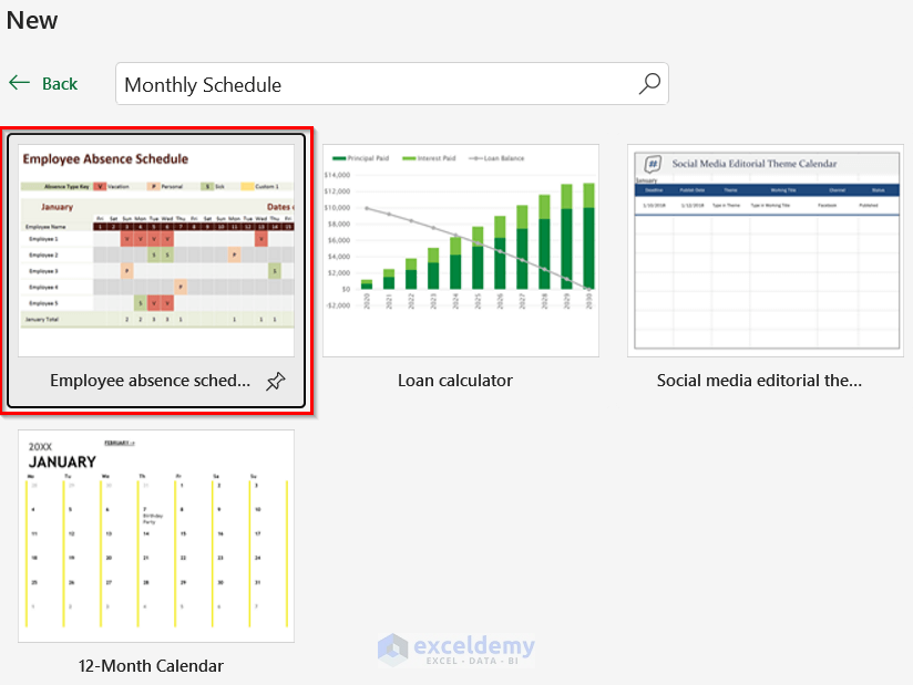
Several Excel Templates will appear. Choose any sheet according to requirement. We chose the Employee absence schedule.

Click on the Create button.

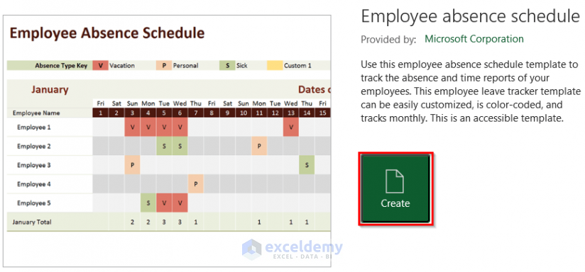
A Monthly Schedule table will open.

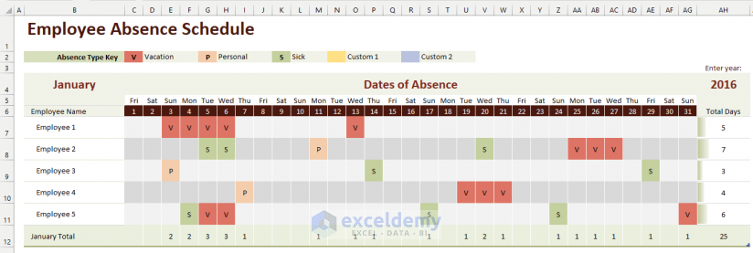
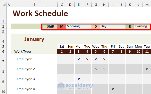
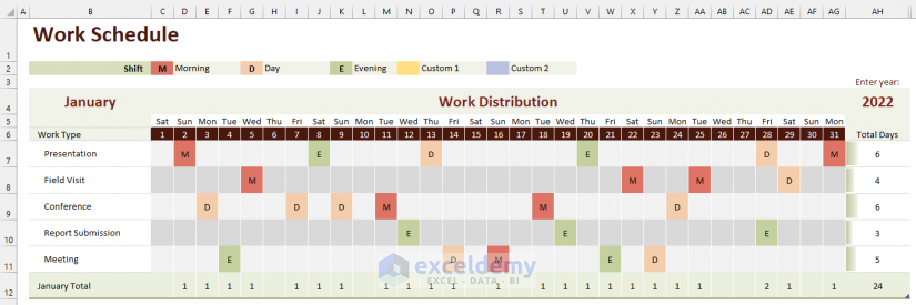
The above image is of an Employee Absence Schedule. You can edit it according to your schedule.

Step 2 – Change Titles

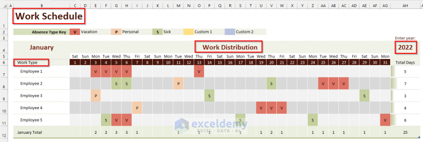
Type Work Schedule in cell B1 and change the titles Dates of Absence to Work Distribution and Employee Name to Work Type.
We inserted 2022 in the Enter year.

Step 3 – Use Data Validation Feature

Discard the entries and add new data in Cell range B7:B11.

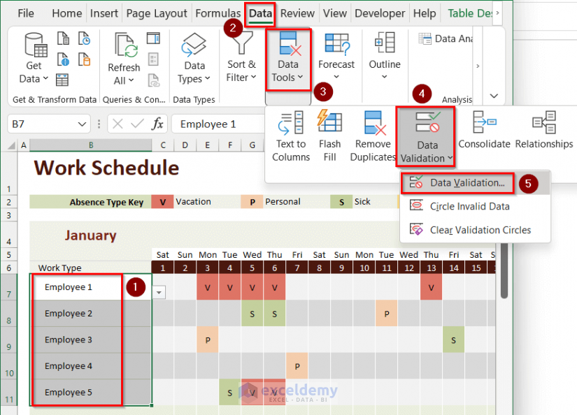
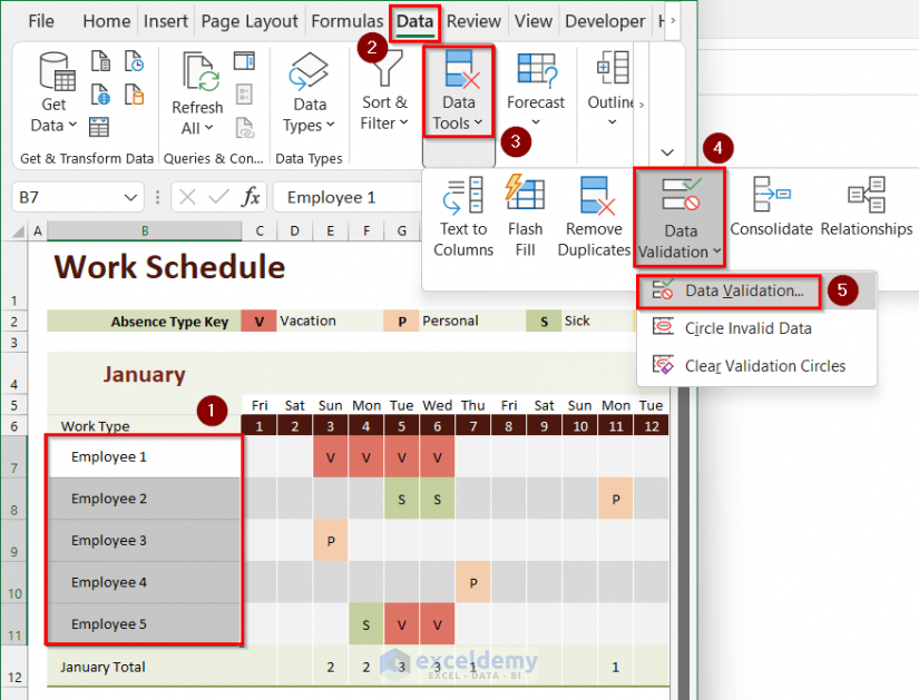
Select cell range B7:B11.
Go to the Data tab >> click on Data Tools >> click on Data Validation >> select Data Validation.

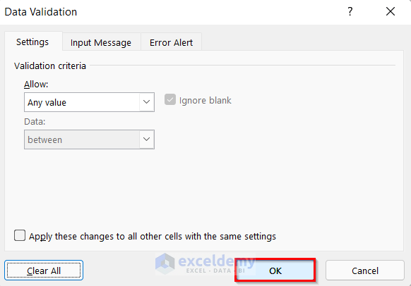
The Data Validation box will pop up.
Click on Clear All.

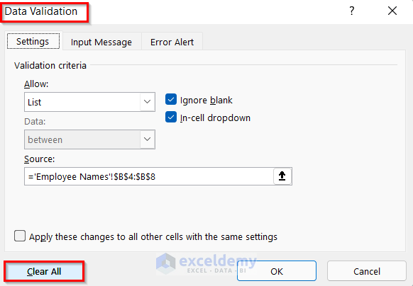
Click on OK.

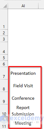
Insert values that you want to add to those cells using the Data Validation feature in any other cell range. We added different work types in cell range AI7:AI11.

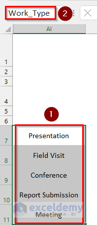
Select cell range AI7:AI11.
Go to the Name box and Type Work_Type.
Press ENTER.

Select cell range B7:B11.
Go to the Data tab >> click on Data Tools>> click on Data Validation >> select Data Validation.

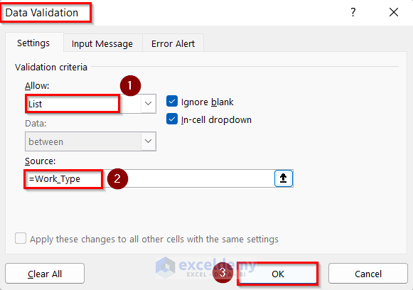
The Data Validation box will pop up.
Select List from the Allow drop-down >> select Work_Type as Source.
Click OK.

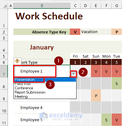
Select cell B7.
Click on the Button shown below.
Select any option of your choice. We selected Presentation.

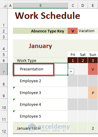
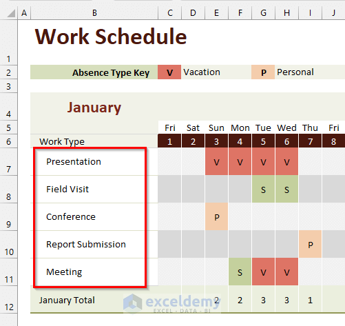
Add data in cell range B8:B11.

Step 4 – Change Values for Creating Monthly Schedule

Change the values of cell range B2:M2 by typing the desired fields. We have typed Shift in Cell B2 and Morning, Day and Evening as new fields and M, D and E as representation.

Select the cell range that contains the schedule for the whole month.
Click on the Delete button.

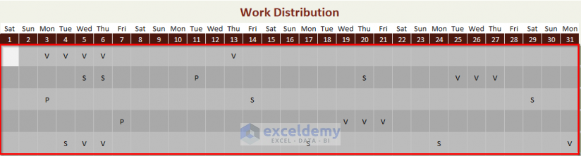
Insert M, D, and E as inputs of the schedule according to your preference.

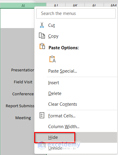
Step 5 – Hide Column

Click on the column you want to hide and Right-click on it.

Click on Hide.

You can now create your own Monthly Schedule based on your preferences.

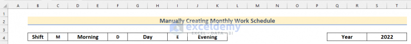
Method 2 – Manually Creating Monthly Work Schedule in Excel

Step 1 – Create Dates in Month

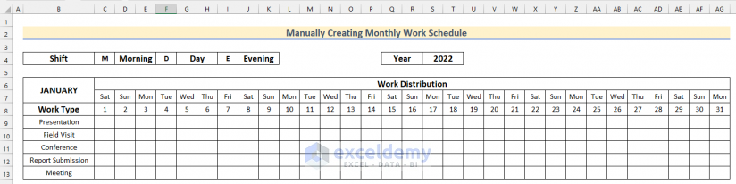
Insert the Shift (or the Fields you want to add) and Year to create a monthly work schedule in Excel.

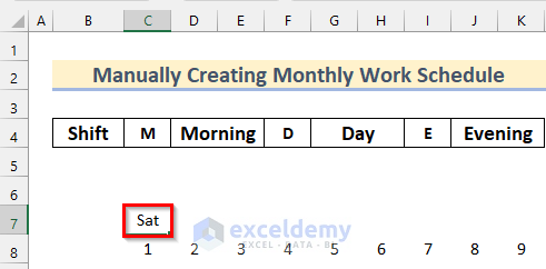
Insert 1 in Cell C8.

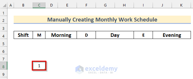
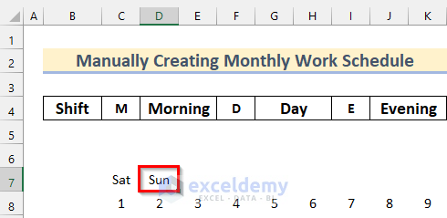
Insert 2 in Cell D8.

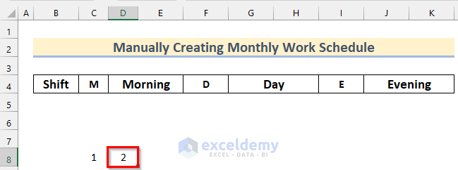
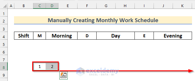
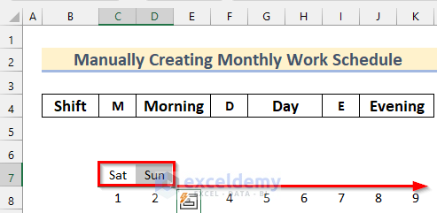
Select Cell C8 and Cell D8.
Drag right the Fill Handle tool to add dates up to 31 of a month.

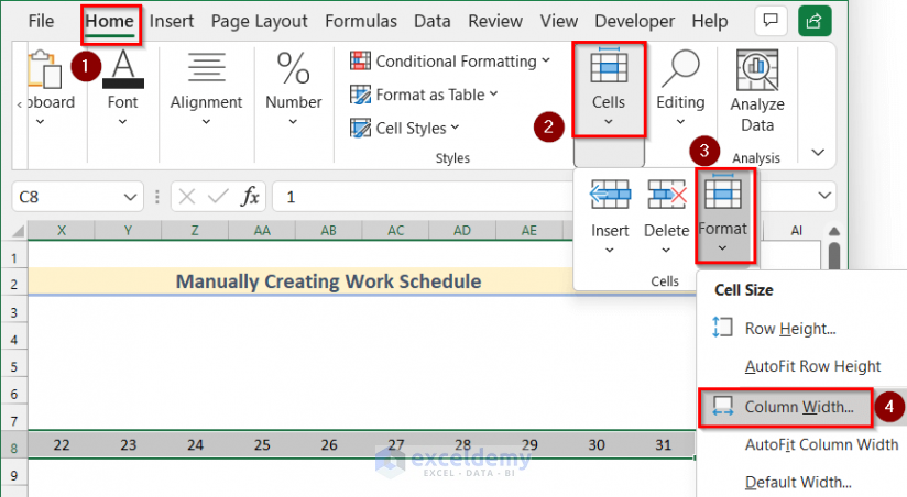
Select Cell range C8:AG8.
Go to the Home tab >> click on Cells >> click on Format >> select Column Width.

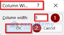
The Column Width box will pop up.
Insert 5 as Column width.
Click on OK.

Insert Sat in Cell C7.

Insert Sun in Cell D7.

Select cell C7 and cell D7.
Drag right the Fill Handle tool to AutoFill the days of the week.

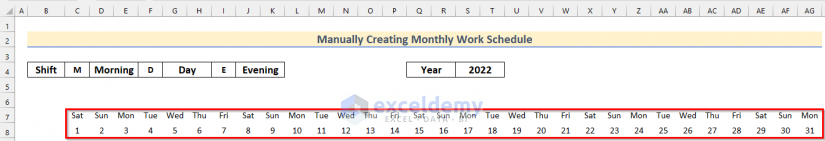
You will get all the days of a month as shown in the image

Step 2 – Insert Titles

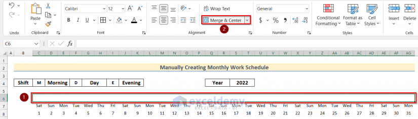
Select cell range C6:AG6.
Click on Merge & Center from the Home.

Type your preferred title.
Press ENTER.
Go to the Home tab >> select 14 as Font Size and click on the Bold button.

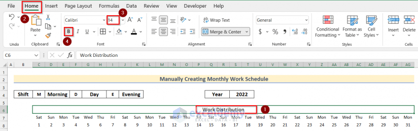
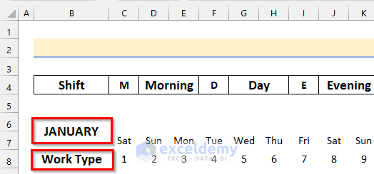
JANUARY and Work Type are added as titles.

Step 3 – Use Data Validation Feature to Create Work Type Drop-Down

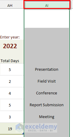
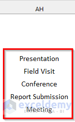
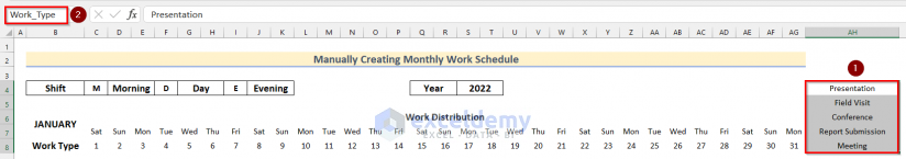
Add different fields to the schedule in a specific column. We added Presentation, Field Visit, Conference, Report Submission and Meeting as Work types in cell range AH4:AH8.

Select cell range AH4:AH8.
Go to the Name box and type Work_Type.
Press ENTER.

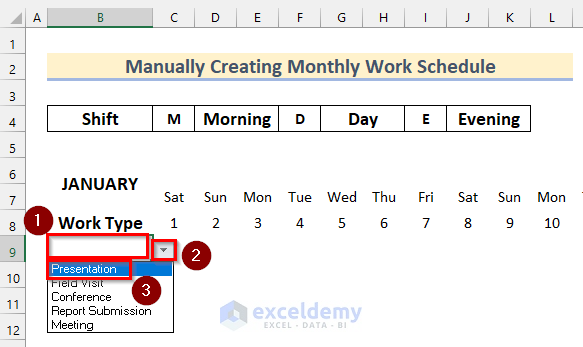
Create a drop-down button in cell B9 using the Data Validation feature.
Select cell B9.
Click on the drop-down button.
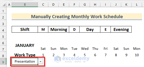
Select any option from the drop-down button. We selected Presentation.

Add values to the rest of the cells.

Step 3 – Format the Dataset

Select cell range B6:AG13.
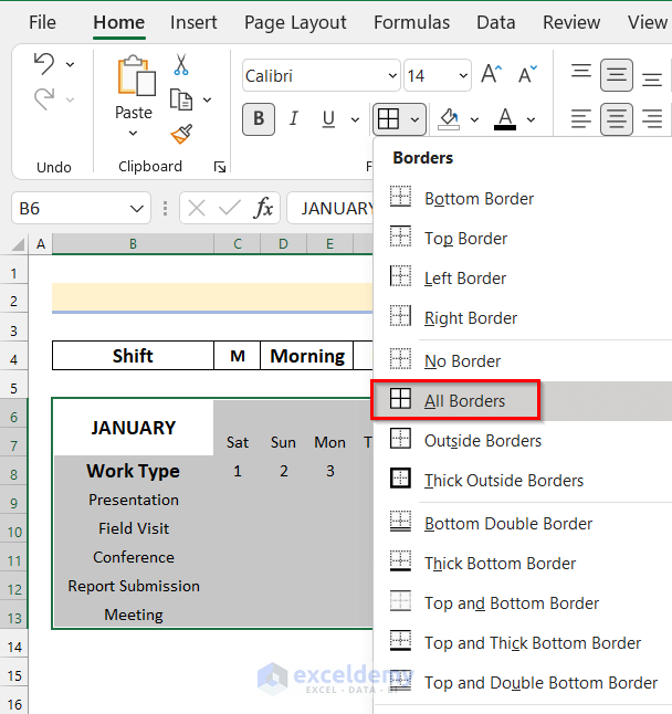
Click on the Borders button from the Home.

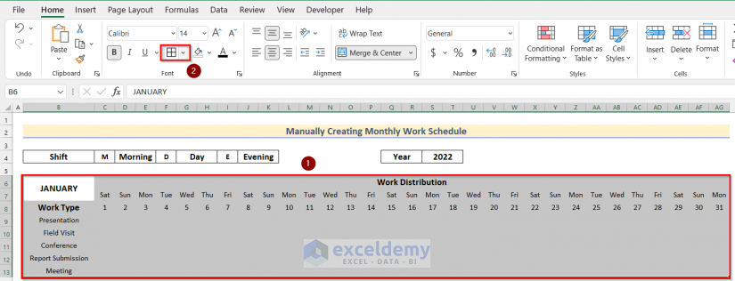
Select All Borders.

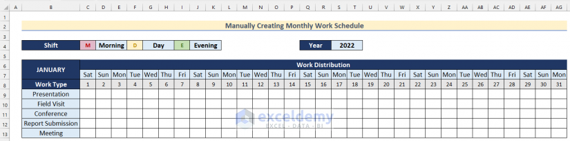
The dataset will look like the image below.

Format the dataset using Fill Color and Font Color.

Step 4 – Insert Data and Using Conditional Formatting

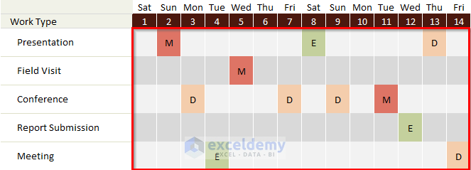
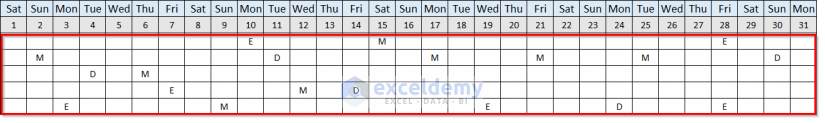
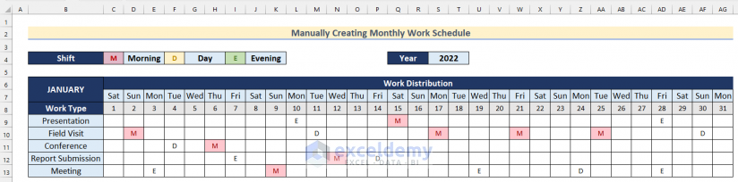
Insert M, D, and E as the short form of Morning, Day and Evening shifts in cell range C9:AG13.

Select cell range C9:AG13.
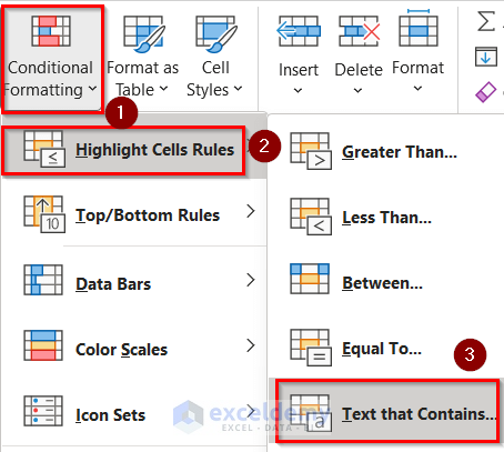
Go to the Home tab >> click on Conditional Formatting.

Click on Highlight Cells Rules>> select Text that Contains.

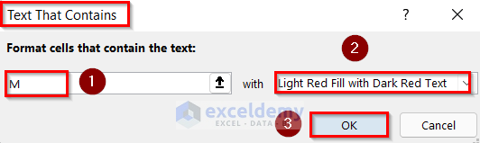
TheText That Contains box will pop up.
Insert M in the box and choose Light Red Fill with Dark Red Text as a format.
Click on OK.

The dataset will look like this.

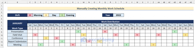
Use Conditional Formatting for the other shifts.

Method 3 – Using Combo Box to Create Monthly Schedule in Excel

Step 1 – Insert a Combo Box

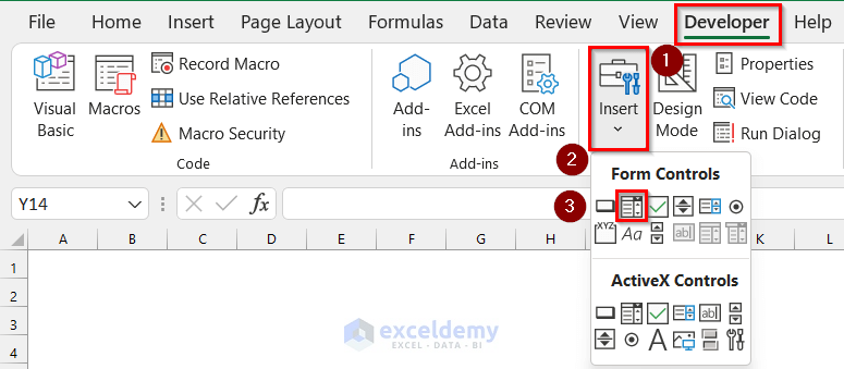
Go to the Developer tab >> click on Insert >> select Combo Box from Form Controls.

Insert a Combo Box in Cell B4.

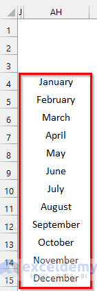
Type the value of 12 months in cell range AH4:AH15.

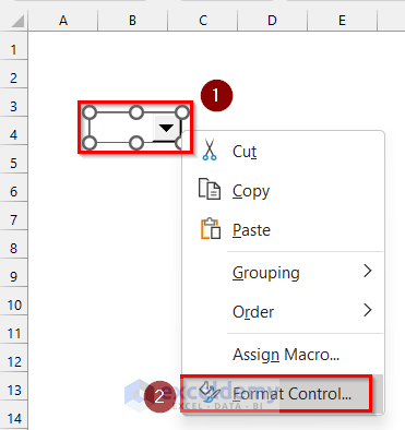
Select the Combo box and Right-click on it.
Click on Format Control.

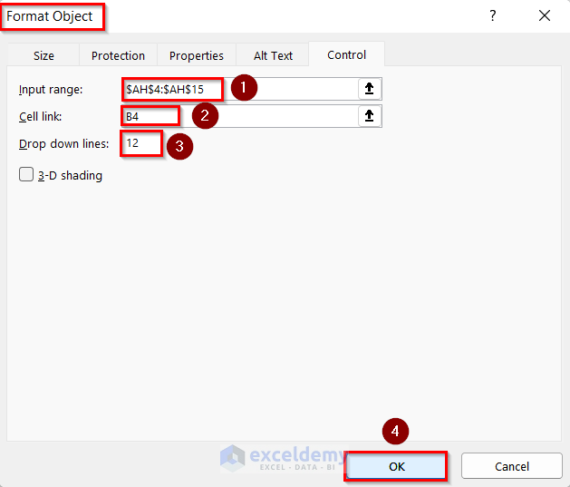
The Format Object box will pop up.
Insert cell range AH4:AH15 as Input range, cell B4 as Cell link and 12 as Drop down lines.
Click on OK.

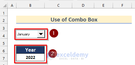
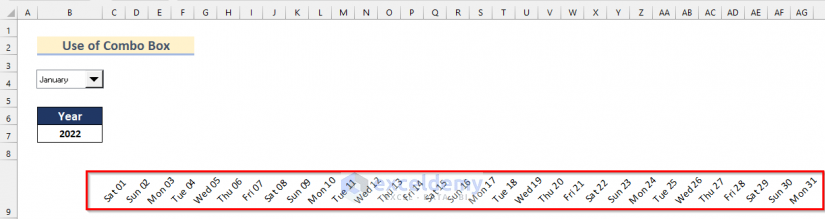
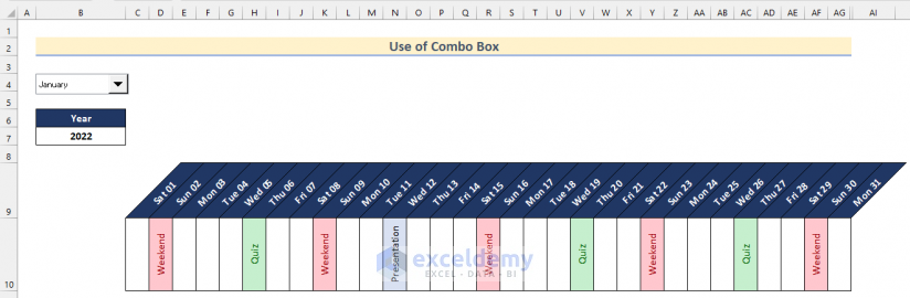
Select any month from the drop-down list. We selectedJanuary.
Add the year in cell B7.
Hide Column AH.

Step 2 – Add Dates to Create a Monthly Schedule

Select cell C9.
Insert the following formula.

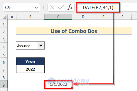
=DATE(B7,B4,1)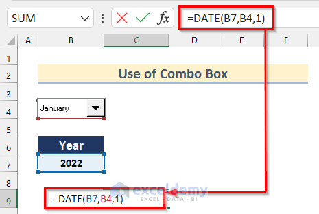

In the DATE function, we inserted Cell B7 as year, Cell B4 as month, and 1 as day.

Press ENTER.

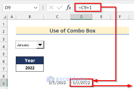
Select cell D9 and insert the following formula.

=C9+1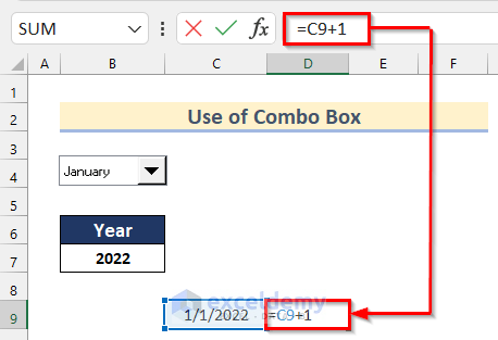

Press ENTER.
Drag down the Fill Handle tool to AutoFill the formula.

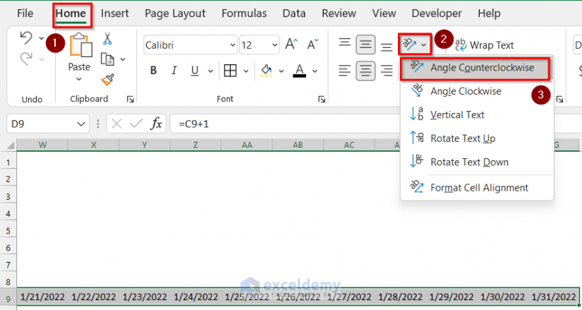
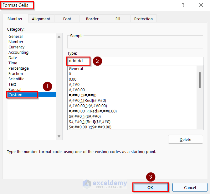
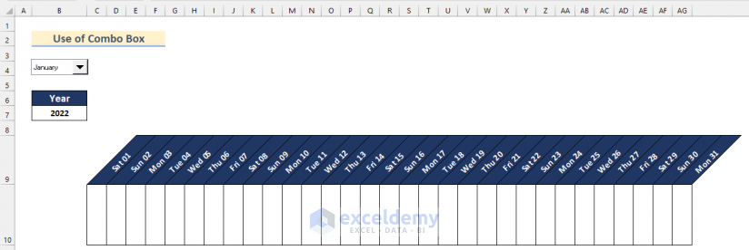
Step 3 – Format Cells

Select cell range C9:AG9.
Go to the Home tab >> click on Orientation >> select Angle Counterclockwise.

Click on Row 9 and Right-click on it.

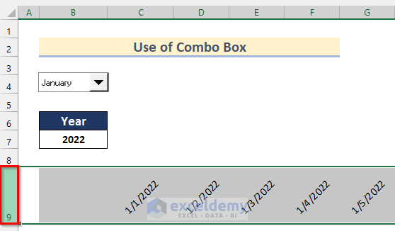
Click on Format Cells.

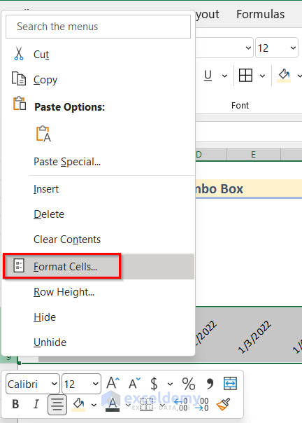
The Format Cells box will pop up.
Go to the Custom option >> Type ddd dd in the box.
Click on OK.

Change the Column Width of Cell range C9:AG9.

Format Cell range C9:AG10 to create a monthly schedule. We used Cell range C10:AG10to add fields to the monthly schedule.

Step 4 – Insert Values for Creating Monthly Schedule

Add different works or fields in cell range C10:AG10. We added Weekend, Quiz and Presentation.

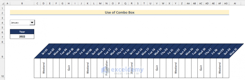
Use Conditional Formatting to highlight these Cells going through the same steps shown in Method 2.

How to Create Monthly Time Schedule in Excel

Step 1 – Use Name Box and Data Validation Feature

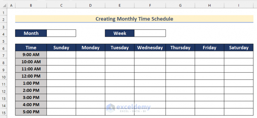
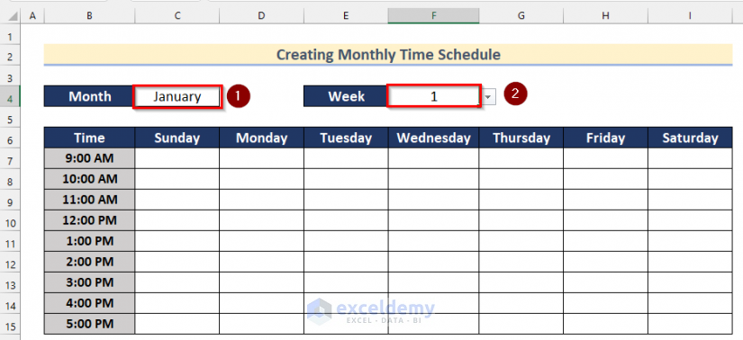
Create a dataset with formatting as shown in the image.

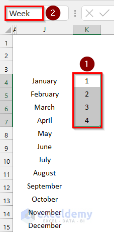
Insert the value of the months in cell range J4:J15 and the value of week numbers in cell range K4:K7.

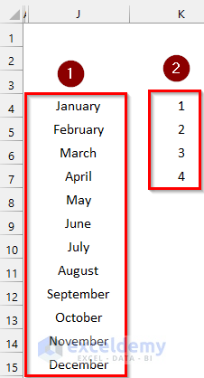
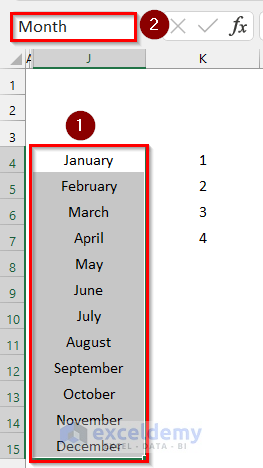
Select cell range J4:J15.
Go to the Name box and type Month.
Press ENTER.

Select cell range K4:K7.
Go to the Name box and type Week.
Press ENTER.

Insert the value of the month in cell C4 and the week number in cell F4 using two drop-down buttons created by using the Data Validation feature.
Hide Column J and Column K.

Step 2 – Insert Values for Creating Monthly Schedule

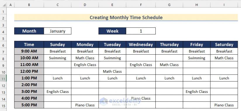
Insert values in cell range C7:I15 to create a schedule. We inserted Breakfast, Lunch, Swimming, English Class, Math Class, and Piano Class as work to do in the schedule.

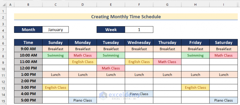
Use Conditional Formatting to highlight these Cells going through the same steps shown in Method 2.

Download Practice Workbook

Create Monthly Schedule.xlsm

Free Template.

Work Schedule Using Excel Templates.xlsx

Related Articles

<< Go Back to Excel for Business | Learn Excel

Get FREE Advanced Excel Exercises with Solutions!

SaveSavedRemoved 0

Tags: Make Schedule in Excel

Arin Islam

Anowara Islam Arin, a graduate of Civil Engineering from Khulna University of Engineering & Technology, Bangladesh, serves as a technical content creator in the ExcelDemy project. Possessing a passion for innovation and critical thinking, she actively embraces challenges. Beyond her engineering background, Arin exhibits a keen interest in Excel, having authored numerous articles on Excel & VBA-related issues to simplify the experience for users facing obstacles in Excel. Besides, she is also interested in Advanced Excel,... Read Full Bio

We will be happy to hear your thoughts

Leave a reply Cancel reply

Submit Excel Problem