How to Display the Equation of a Line in an Excel Graph (2 Easy Ways)

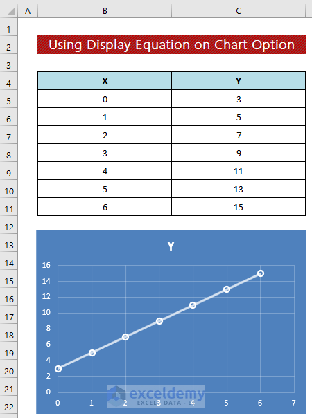
Here’s the dataset we’ll use to explore the methods. We made the line graph using the equation y = 2x + 3.

Method 1 – Using Display Equation in Chart Option to Show the Equation of a Line

Steps:

• Click anywhere on the chart, and you will get three icons beside the right side of the chart
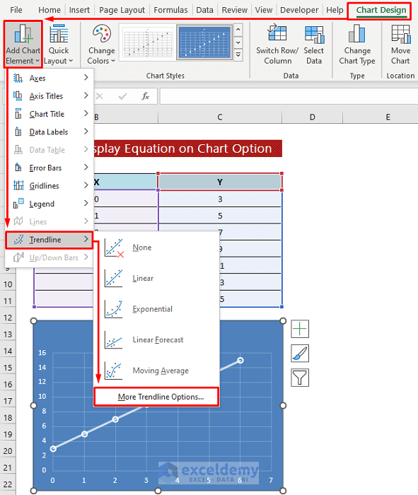
• Click on the Chart Element icon from the right side of the chart.
• Choose Trendline > More Options.

• Click as follows from the Chart Design ribbon: Add Chart Element > Trendline > More Trendline Options.
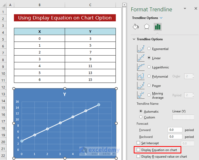
• The fastest way is to just double-click on the line of the chart.

The Format Trendline field will appear on the right side of your Excel window.

• Mark the Display Equation on Chart option from the field.

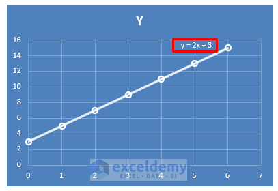
The equation appeared in the chart.

Read More: How to Graph Two Equations in Excel

Method 2 – Displaying the Equation of a Line in Excel Graph Manually

2.1. Inserting Text Box

Steps:

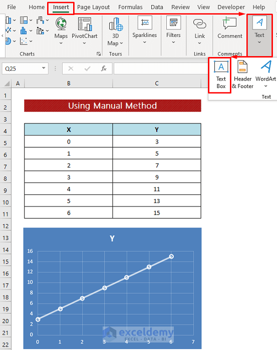
• Go to the Insert ribbon and click on the Text Box command from the Text

Your cursor will look like this:

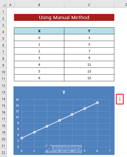
• Click, hold, and drag over anywhere on the sheet to make a box.

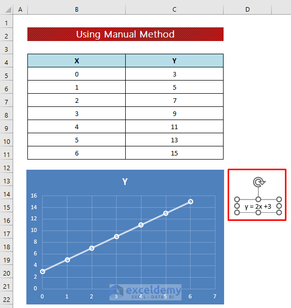
• Enter the equation in the box.

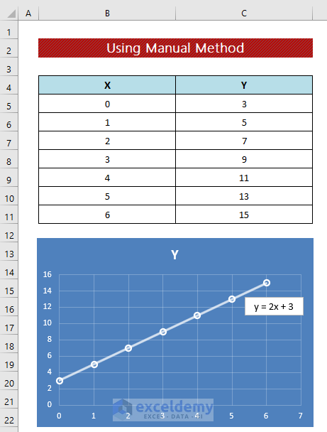
• Insert the box on the chart.

It looks like the output of the previous method.

Read More: How to Graph a Linear Equation in Excel

2.2. Insert an Equation

Steps:

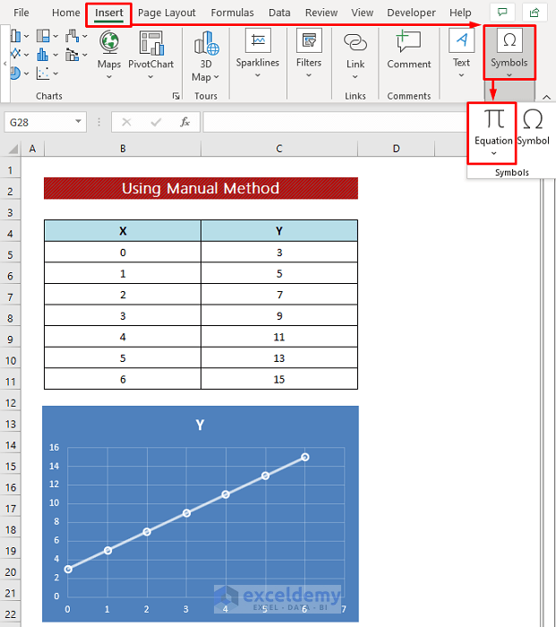
• Click on the Insert ribbon.
• Click Equation from the Symbols

You will get an equation box like the image below.

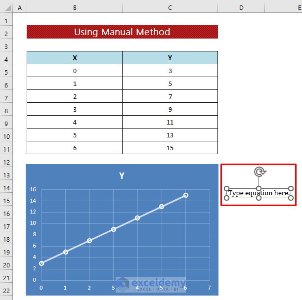
• Type the equation in the box.

You can change the format. We applied the center and middle alignment here again.

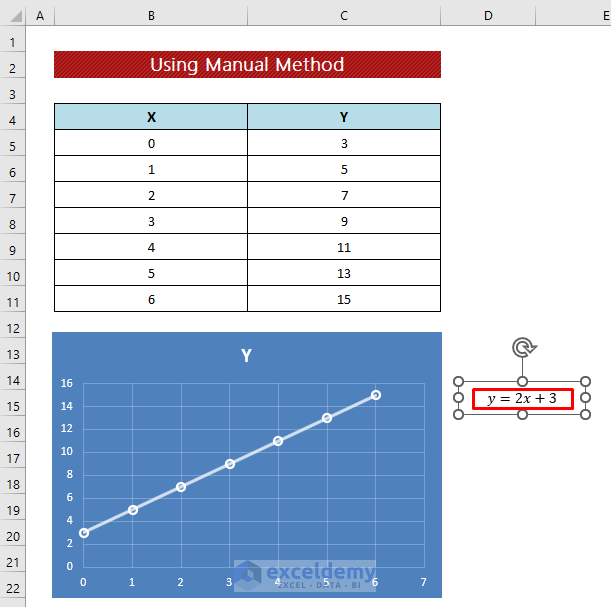
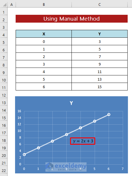
• Insert the equation box on the chart by dragging.

The equation box’s outlook is much better than the text box.

Read More: How to Graph an Equation in Excel Without Data

Download the Practice Workbook

You can download the free Excel workbook from here and practice.

<< Go Back to Plot an Equation | Excel Charts | Learn Excel