A simple linear equation: y = mx + c will be used. This equation will return straight lines when plotted on a graph. Here, x is an independent variable, whereas y depends on x. c is a constant, known as the intercept of y. m is the gradient, also known as the slope of the straight line.
To graph the equation without a dataset:
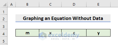
STEP 1 – Input Equation
- Enter m, x, c, and y in B4:E4.
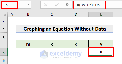
STEP 2 – Apply a Formula for Calculation
Create a formula to calculate the y variable.
- In E5, use the formula:
=(B5*C5)+D5- Press Enter.
It’ll return 0.
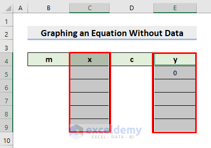
STEP 3 – Graph Equation
Insert a graph:
- Select C4:C9.
- Press and hold Ctrl.
- Select E4:E9.
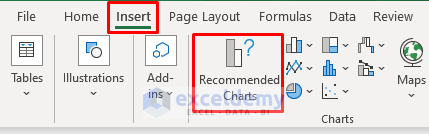
- Go to the Insert tab.
- Click Recommended Charts.
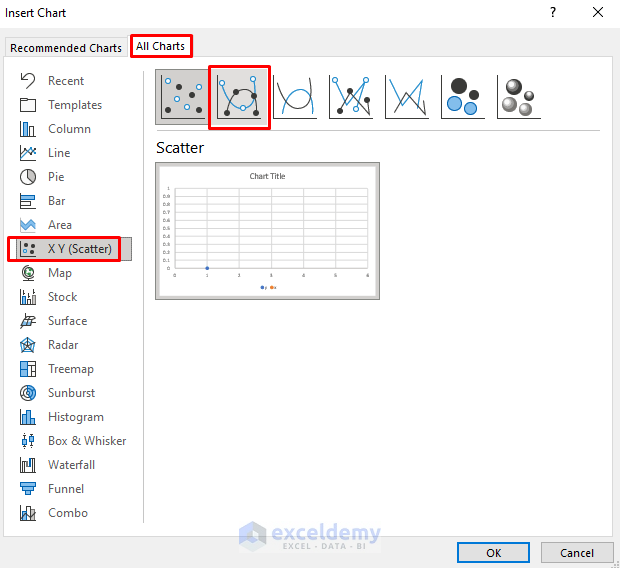
- In the Insert Chart dialog box, select All Chart.
- Click X Y (Scatter).
- Choose Scatter with Smooth Lines and Markers.
- Click OK.
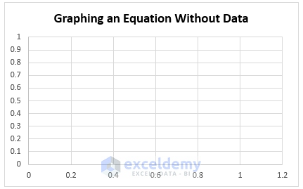
- The graph is displayed (as the dataset is empty, you won’t see any plottings).
STEP 4 – Enter Data
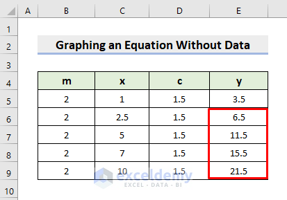
- Enter the value of m as 2.
- Enter values for the independent variable x.
- Enter the value of c as 5.
- Drag down the Fill Handle to see the result in the rest of the cells.
- The output for y will be returned.
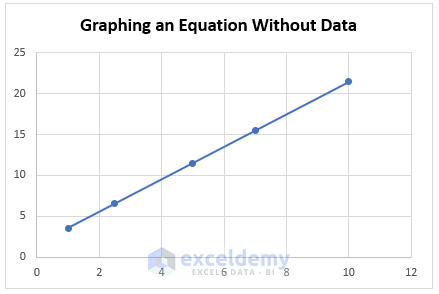
Final Output
A linear line graph will be displayed as shown below.
Read More: How to Graph a Linear Equation in Excel
Download Practice Workbook
Download the following workbook.
Related Articles
<< Go Back to Plot an Equation | Excel Charts | Learn Excel
Get FREE Advanced Excel Exercises with Solutions!
