Method 1 – Use Only COUNTIF Function to Compare Two Columns in Excel
Steps:
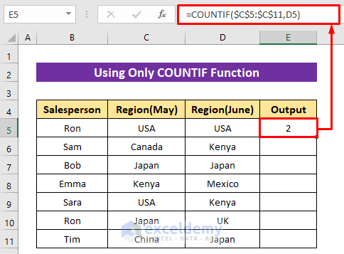
- Type the following formula in Cell E5–
=COUNTIF($C$5:$C$11,D5)- Hit the Enter button for the output.
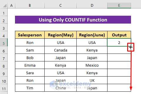
- Use the Fill Handle tool to copy the formula for the other cells of the column.
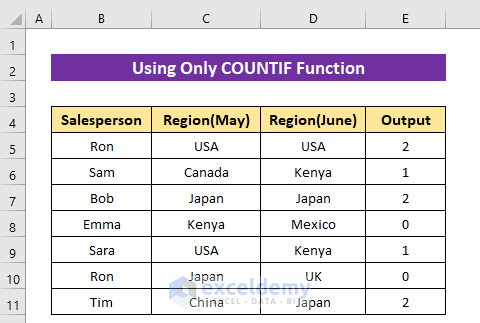
Get the match number for every value like the image below.
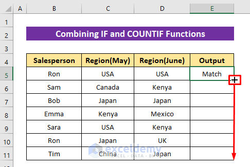
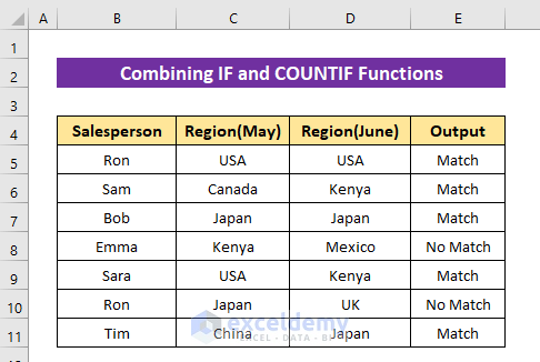
Method 2 – Combine IF and COUNTIF Functions to Compare Two Columns
Steps:
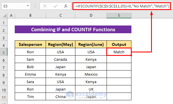
- Insert the following formula in Cell E5–
=IF(COUNTIF($C$5:$C$11,D5)=0,"No Match","Match")- Press the Enter button to return the first output.
Formula Breakdown:
- COUNTIF($C$5:$C$11,D5)=0
The COUNTIF function will count the match number for every value of Column D from Column C. If it gets equal to zero then will return TRUE otherwise FALSE.
- IF(COUNTIF($C$5:$C$11,D5)=0,”No Match”,”Match”)
The IF function will return ‘No Match’ for TRUE and ‘Match’ for FALSE.
- Get the other output, use the Fill Handle tool.
The formula returns the desired output.
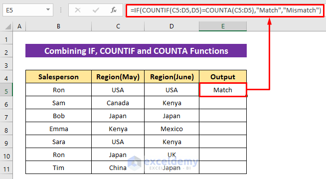
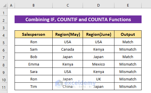
Method 3 – Merge IF, COUNTIF and COUNTA Functions to Compare Two Columns
Steps:
- In Cell E5, write the following formula-
=IF(COUNTIF(C5:D5,D5)=COUNTA(C5:D5),"Match","Mismatch")- Hit the Enter button for the result.
Formula Breakdown:
- COUNTA(C5:D5)
The COUNTA function will count cells from the range of the row.
- COUNTIF(C5:D5,D5)
The COUNTIF function will count the match from the row based on the value of the second column.
- COUNTIF(C5:D5,D5)=COUNTA(C5:D5)
This logical test will happen to check whether it is TRUE or FALSE.
- IF(COUNTIF(C5:D5,D5)=COUNTA(C5:D5),”Match”,”Mismatch”)
Finally, the IF function will return ‘Match’ for TRUE and ‘Mismatch’ for FALSE.
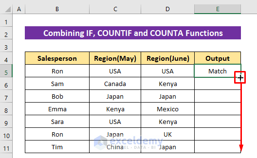
- Apply the Fill Handle icon for the output of the rest of the cells.
The final output of the comparison based on each row.
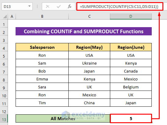
Method 4 – Combine COUNTIF and SUMPRODUCT Functions to Compare Two Columns
Steps:
- Insert the following formula in Cell D13–
=SUMPRODUCT(COUNTIF(C5:C11,D5:D11))- Hit the Enter button, and it will return 5 for our dataset.
Formula Breakdown:
- COUNTIF(C5:C11,D5:D11)
The COUNTIF function will check if each value from Column C matches Column A. If matches then 1 will return, otherwise will return 0. It will return the output as an array- {1;1;0;1;0;1;1}
- SUMPRODUCT(COUNTIF(C5:C11,D5:D11))
The SUMPRODUCT function will sum up all the values from the array and will return 5.
Download Practice Workbook
You can download the free Excel workbook from here and practice independently.
Related Articles
- How to Use COUNTIF Function in Excel Greater Than Percentage
- Excel COUNTIF to Count Cells Greater Than 1
- How to Use COUNTIF for Non Contiguous Range in Excel
- How to Use COUNTIF Function to Calculate Percentage in Excel
- How to Use COUNTIF Function with Array Criteria in Excel
- How to Calculate Frequency Using COUNTIF Function in Excel
<< Go Back to Excel COUNTIF Function | Excel Functions | Learn Excel
Get FREE Advanced Excel Exercises with Solutions!
