Method 1 – Using COUNTIF Function to Calculate Frequency in Excel
Steps:
- Use the following formula in cell D17.
=COUNTIF($C$5:$C$14,"<="&B17)The range of cells $C$5:$C$14 indicates the array of the Marks obtained by the students, and cell B17 refers to the 1st cell of the Number column.
- Press ENTER.
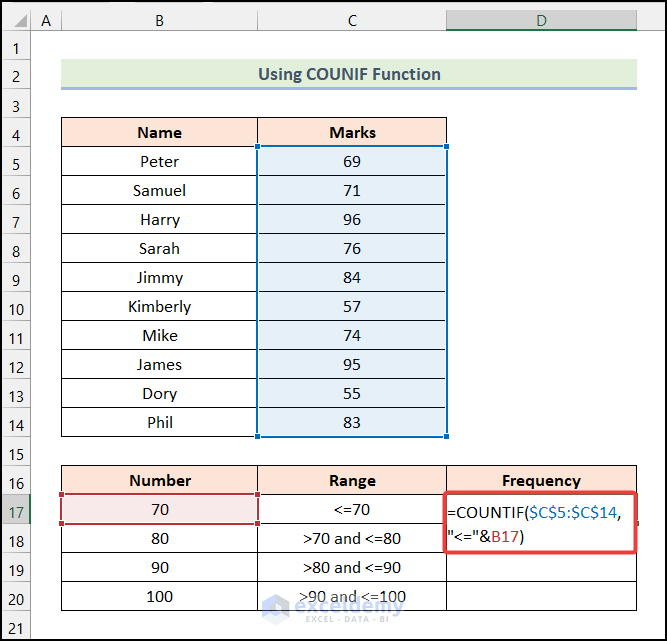
You will have the frequency of Marks, which is less than or equal to 70 in cell D17.

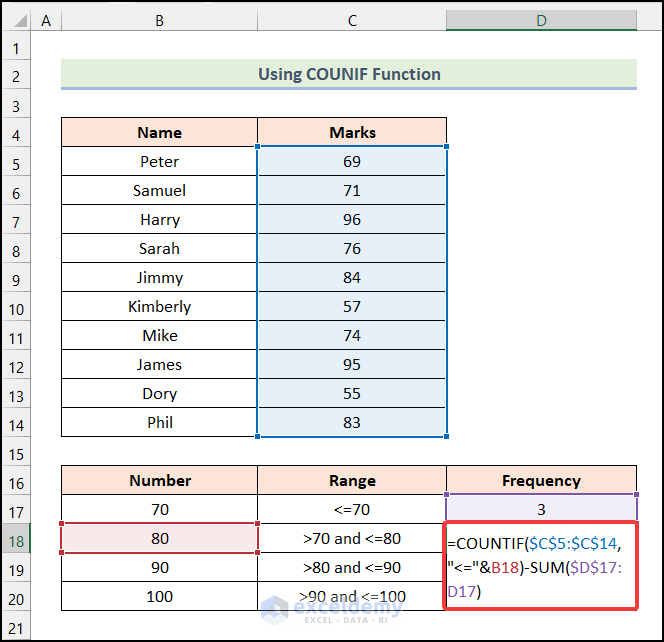
- Enter the formula given below in cell D18.
=COUNTIF($C$5:$C$14,"<="&B18)-SUM($D$17:D17)Cell B18 indicates the 2nd cell of the Number column, and range $D$17:D17 represents the cells of the Frequency column.
Formula Breakdown
- COUNTIF($C$5:$C$14,”<=”&B18)
- Here, $C$5:$C$14 → It is the range argument.
- “<=”&B18 → This refers to the criteria argument,
- Output → 6.
- SUM($D$17:D17) → Returns the sum of the range $D$17:D17.
- Output → 3.
- COUNTIF($C$5:$C$14,”<=”&B18)-SUM($D$17:D17) → 6-3.
- Output → 3.
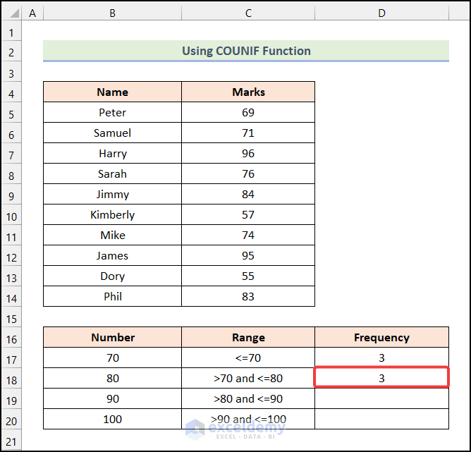
- Hit ENTER.
You will have the frequency of Marks greater than 70 and less than or equal to 80 in cell D18, as shown in the following image.
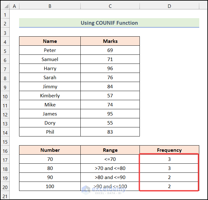
- Use the AutoFill option of Excel to get the rest of the outputs as demonstrated in the following picture.
Method 2 – Calculating Frequency for Texts with Excel COUNTIF Function
Steps:
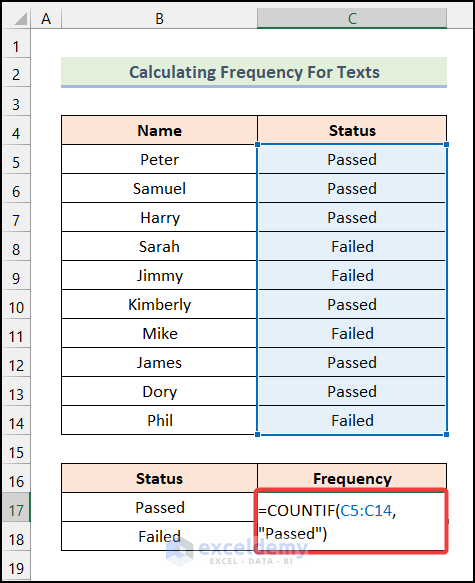
- Apply the formula given below in cell C17.
=COUNTIF(C5:C14,"Passed")The range of cells C5:C14 refers to the cells of the Status column.
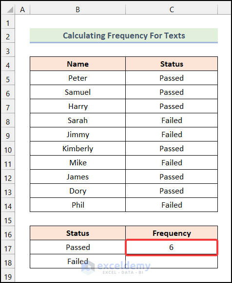
- Press ENTER.
You will have the number of students that get “Passed” status in the exam (see cell C17).
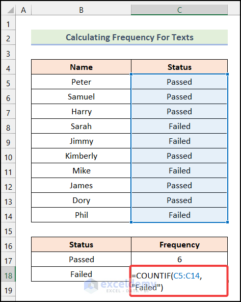
- Enter the following formula in cell C18.
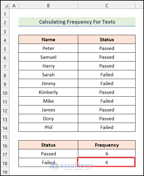
=COUNTIF(C5:C14,"Failed")- Hit ENTER.
You will have the following output on your worksheet, as shown in the image below.
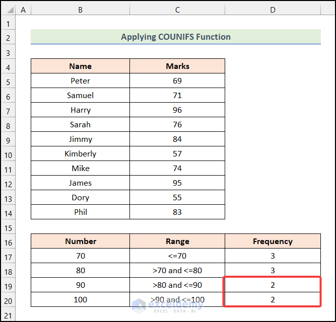
How to Count Frequency Using COUNTIFS Function in Excel
Steps:
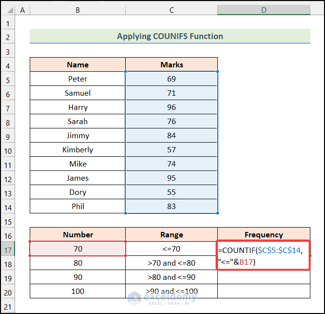
- Use the following formula in cell C17.
=COUNTIF($C$5:$C$14,"<="&B17)- Press ENTER.
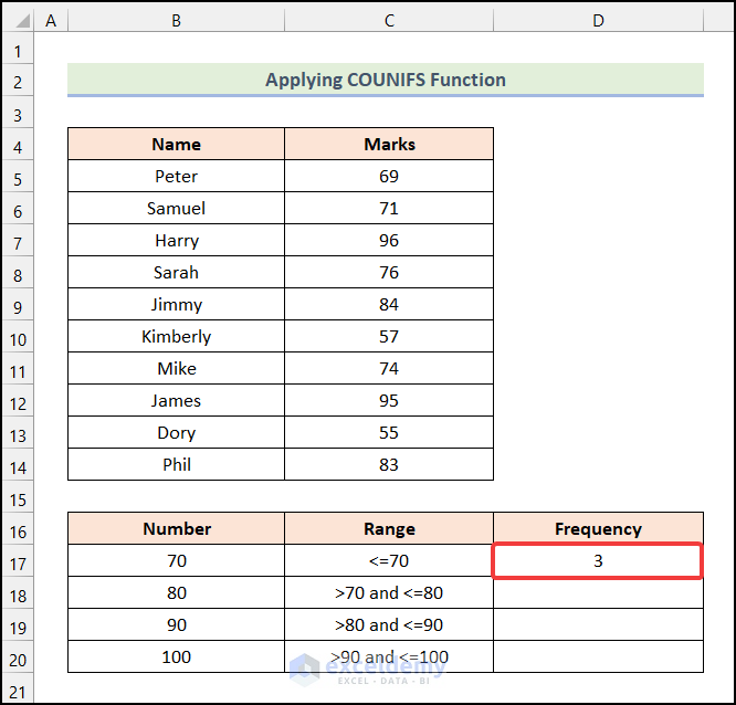
You will see the following output on your worksheet.
- Apply the formula given below in cell C18.
=COUNTIFS($C$5:$C$14,">"&B17,$C$5:$C$14,"<="&B18)- Hit ENTER.
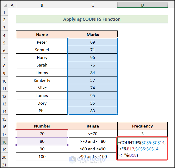
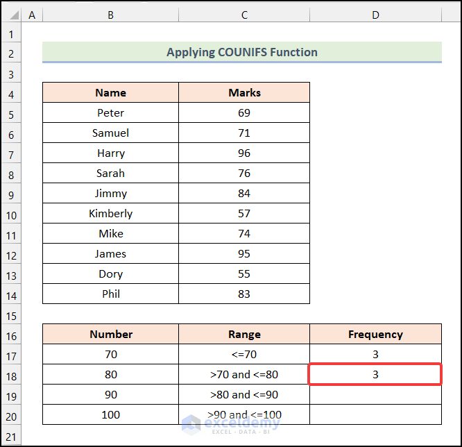
You will have the frequency of Marks that are greater than 70 but less than or equal to 80 in cell C18.
- Use Excel’s AutoFill feature to get the rest of the frequencies, as demonstrated in the following image.
How to Find Frequency of a Range in Excel
Steps:
- Use the following formula in cell D17.
=FREQUENCY(C5:C14,B17:B20)The range of cells C5:C14 refers to the cells of the Marks column, and B17:B20 indicates the cells of the Bins column.
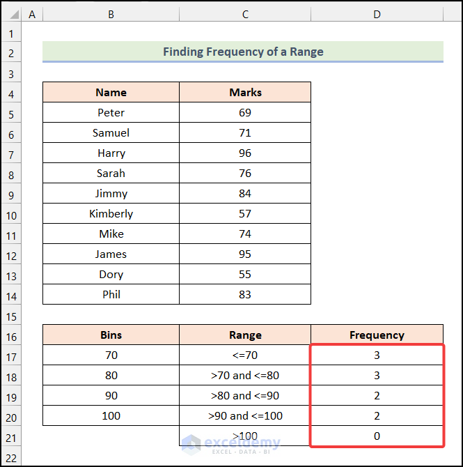
- Press ENTER.
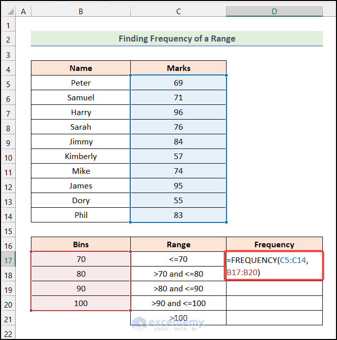
The FREQUENCY function will return the following outputs, as shown in the picture.
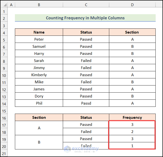
How to Count Frequency of Values in Multiple Columns in Excel
Steps:
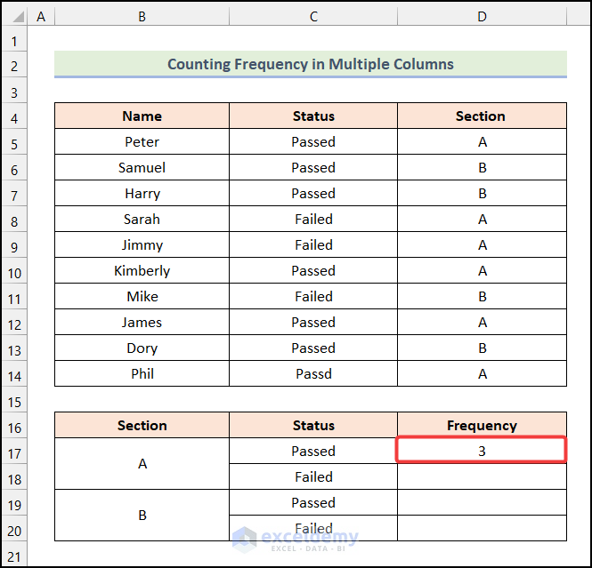
- Use the formula below in cell D17.
=COUNTIFS($D$5:$D$14,$B$17,$C$5:$C$14,C17)The range of cells $D$5:$D$14 represents the cells of the Section column, cell $B$17 indicates the selected Section, and cell C17 represents the selected Status.
- Hit ENTER.
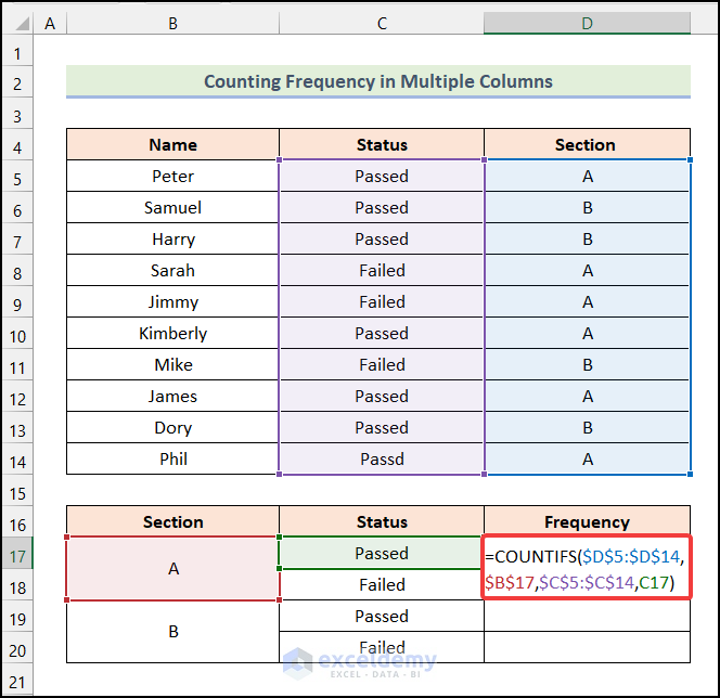
You will have the frequency of the students of “Section A” that get “Passed” status in the exam.
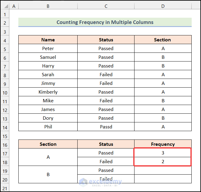
- Drag the Fill Handle to copy down the formula up to cell D18.
You will know the number of the students of “Section A” who gather “Failed” status in the exam.
- Enter the following formula in cell D19.
=COUNTIFS($D$5:$D$14,$B$19,$C$5:$C$14,C17)- Press ENTER.
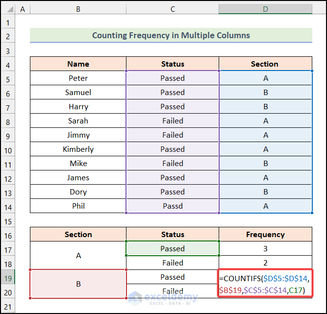
You will have the frequency of the students of Section B that get “Passed” status in the exam in cell D19.
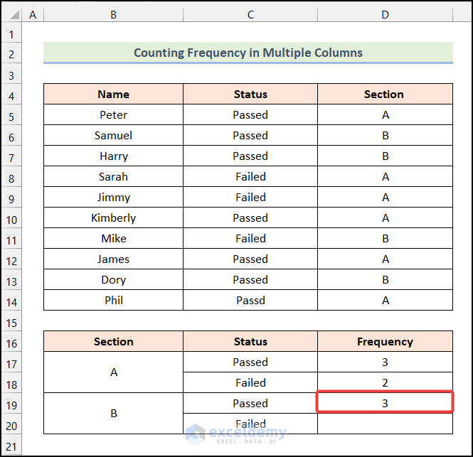
- Drag the Fill Handle up to cell D20 to copy down the formula.
You will get the number of the students of Section B that get “Failed” status in the exam (in cell D20), as demonstrated in the following picture.
Download Practice Workbook
Related Articles
- How to Use COUNTIF Function to Calculate Percentage in Excel
- How to Use COUNTIF Function in Excel Greater Than Percentage
- How to Compare Two Columns Using COUNTIF Function
- How to Use Excel COUNTIF Between Time Range
<< Go Back to Excel COUNTIF Function | Excel Functions | Learn Excel
Get FREE Advanced Excel Exercises with Solutions!
