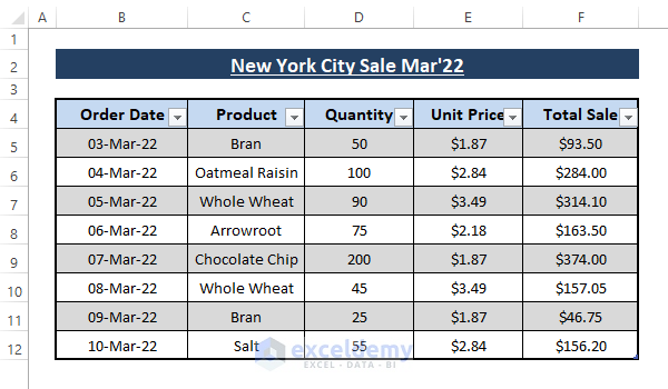
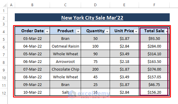
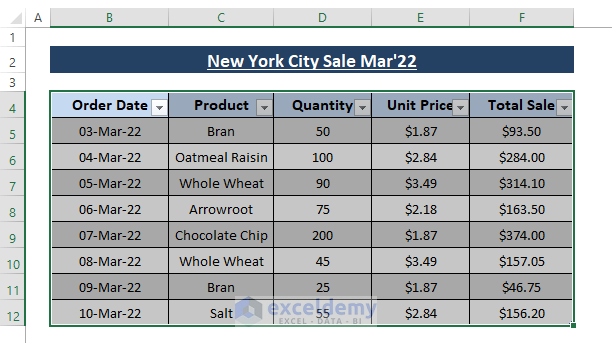
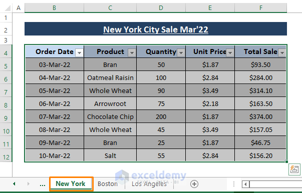
Say we have Sale data in Table format for March’22 for three different cities, New York, Boston, and Los Angeles. These three sets of Sales data are identical in orientation, so we show only one set of sales data as a dataset:
In this article, we’ll use Structured References, Insert Link, and HYPERLINK functions to reference a Table in another Excel sheet.
Before introducing our methods, it’s convenient if we assign specific names to our Tables, so we can simply type their names when referencing them.
STEPS:
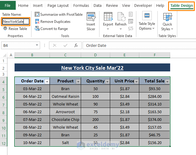
- Select the entire table or place the cursor in any cell of the table.
Excel displays the Table Design tab.
- Click on Table Design.
- Assign a Table name (i.e., NewYorkSale) under the Table Name dialog box in the Properties section.
- Press ENTER.
Excel then assigns the name to this Table.
- Repeat these Steps for the other 2 Tables (BostonSale and LosAngelesSale).
- Check the naming using Formulas > Name Manager (in the Defined Names section).
You will see all the assigned Table names in the Name Manager window.
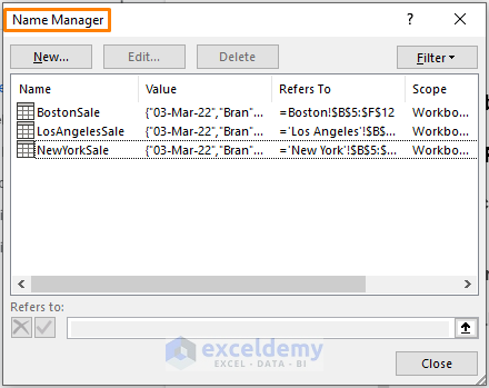
Now we can easily reference them in formulas.
Read More: Types of Tables in Excel: A Complete Overview
Method 1 – Using Structured Reference
Structured Reference means we can reference an entire column by just providing the header name in the formula along with the assigned Table name.
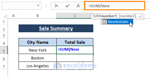
- Start typing a formula after inserting an Equal Sign (=) in the Formula bar.
- Enter a Table name to reference it, as shown in the image below.
- Excel brings up the Table reference; double-click on it.
- After referencing the Table, type a third bracket ([).
Excel shows column names to select from.
- Double-click on Total Sale and close the brackets.
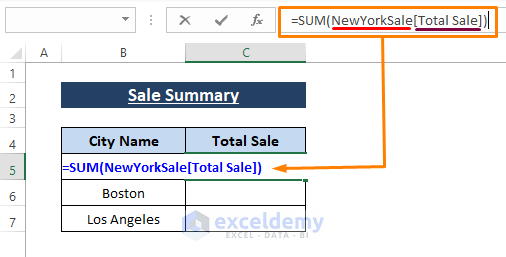
- Assign New York Sale Table, then one of its columns (Total Sale).
Both arguments are indicated in colored rectangles.
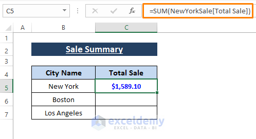
- Press ENTER to apply the formula in cell C5.
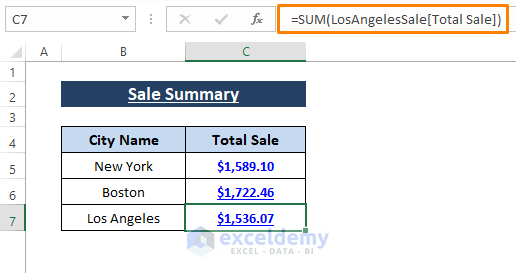
- Follow the steps above to reference the other Tables in the respective cells.
After referencing, Excel shows the sum of the Total Sale columns of the respective Tables as follows:
You can reference any Table just by assigning its name in the formula, along with the column header you want to deal with.
Method 2 – Using Insert Link
Excel’s Insert Link is an effective way to link or reference cells or ranges from other sheets. As we are referencing a Table, we need to use the Table range to reference it by link. Prior to the reference, we have to check the range that our Table occupies, similar to the picture below.
- Place the cursor in the cell (i.e. C5) where you want to insert the reference of the Table.
- Go to Insert > Link > Insert Link.
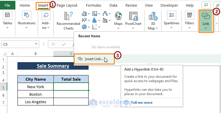
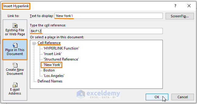
The Insert Hyperlink dialog box opens.
- Click on Place in this Document as the Link to option.
- Select the Sheet (‘New York’) under Or select a place in this document.
- Type cell reference B4:F12 under Type the cell reference.
- Edit or keep what Excel takes as Text to display (i.e. ‘New York’!).
- Click on OK.
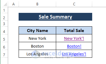
Clicking OK inserts the link of the Table in cell C5.
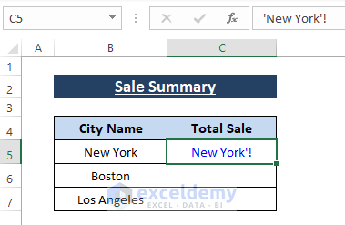
- You can cross-check the referencing just by clicking on the link as shown below.
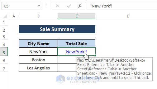
After clicking on the link Excel takes you to the destined worksheet and highlights the entire Table.
- Use the Steps above to insert links for the other Tables (Boston Sale and Los Angeles Sale).
This method is suitable when the table and the sheet name have the same name.
Method 3 – Using the HYPERLINK Function
The HYPERLINK function converts a destination and a given text into a hyperlink. We can then instantly move to a worksheet on demand just by clicking on the links.
The syntax of the HYPERLINK function is:
HYPERLINK (link_location, [friendly_name])In the formula,
link_location; the path to the sheet to which you want to jump.
[friendly_name]; the display text in the cell where we insert the hyperlink [Optional].
Steps:
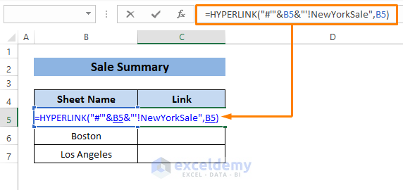
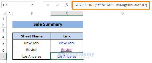
Paste the following formula in cell C5 or any blank cell:
=HYPERLINK("#'"&B5&"'!NewYorkSale",B5)In the formula,
#'”&B5&”‘!NewYorkSale = link_location.
B5 = [friendly_name].
- Press ENTER.
- Insert the same formula in the other cells after replacing the respective Table Names.
Read More: Excel Table vs. Range: What Is the Difference?
Download Excel Workbook
Related Articles
- How to Convert Range to Table in Excel
- Navigating Excel Table
- How to Make Excel Tables Look Good
- How to Convert Table to List in Excel
- Table Name in Excel: All You Need to Know
- How to Create a Table Array in Excel
- How to Insert Floating Table in Excel
- How to Make a Comparison Table in Excel
<< Go Back to Excel Table | Learn Excel
Get FREE Advanced Excel Exercises with Solutions!
