What Is Slicer?
- An Excel slicer is a visual filtering tool that enhances data filtering.
- It is used in conjunction with tables, pivot tables, or pivot charts.
- Slicers provide an easy-to-use interface for filtering data based on predetermined criteria.
- They are developed from one or more fields in a table, pivot table, or pivot chart.
- Slicers are particularly useful when dealing with large datasets, allowing swift filtering and evaluation without manual effort.
- They help users study data, identify trends, and spot patterns effectively.
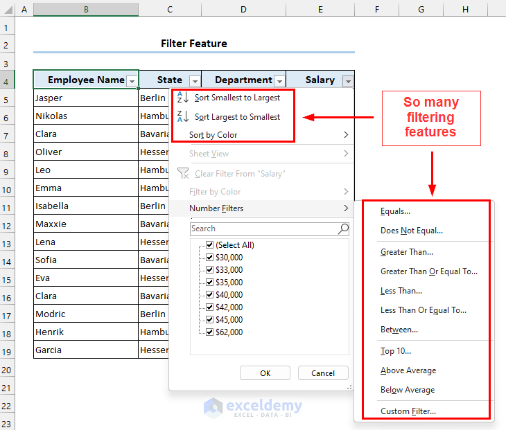
What Is Filter?
- Excel’s filter feature is used to sort, search, and display data based on specific criteria.
- Criteria can include numbers, texts, dates, or other factors.
- Advanced filtering options include sorting data in ascending or descending order and filtering based on a range of values.
- Filters are versatile and can be applied to any type of data in Excel.
Major Differences Between Slicer and Filter
- Application:
- Slicer: Developed for tables, pivot tables, and pivot charts.
- Filter: Applicable to any type of data in Excel.
- User Interface:
- Slicer: Offers an aesthetically pleasing and engaging interface.
- Filter: Uses a drop-down menu or dialog box.
- Criteria:
- Slicer: Allows filtering based on multiple criteria.
- Filter: Filters based on a single criterion at a time.
- Customization:
- Slicer: Provides extensive formatting options (e.g., modifying slicer headers, changing layout colors).
- Filter: Limited customization features.
- Compatibility:
- Slicer: Introduced in Excel 2010; not compatible with versions before 2010.
- Filter: Available in all versions of Microsoft Excel.
- Visibility:
- Slicer: Easier to understand.
- Filter: Can be overwhelming for large spreadsheets.
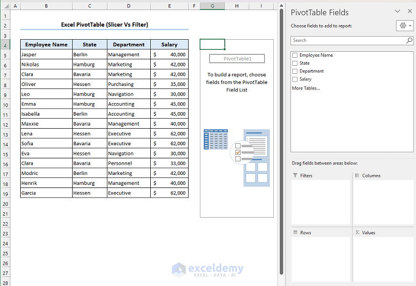
Practical Examples
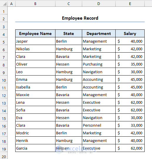
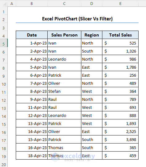
- Let’s consider a dataset representing employees’ records in a company.
- We’ll demonstrate the differences between slicers and filters using an Excel table.
- Suppose we want to filter data related to the Marketing and Executive departments in Bavaria and Hessen states.
- We’ll use both slicer and filter features to compare their effectiveness.
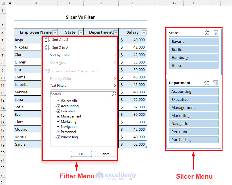
1. Slicer vs Filter in Excel Table
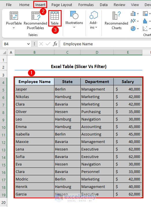
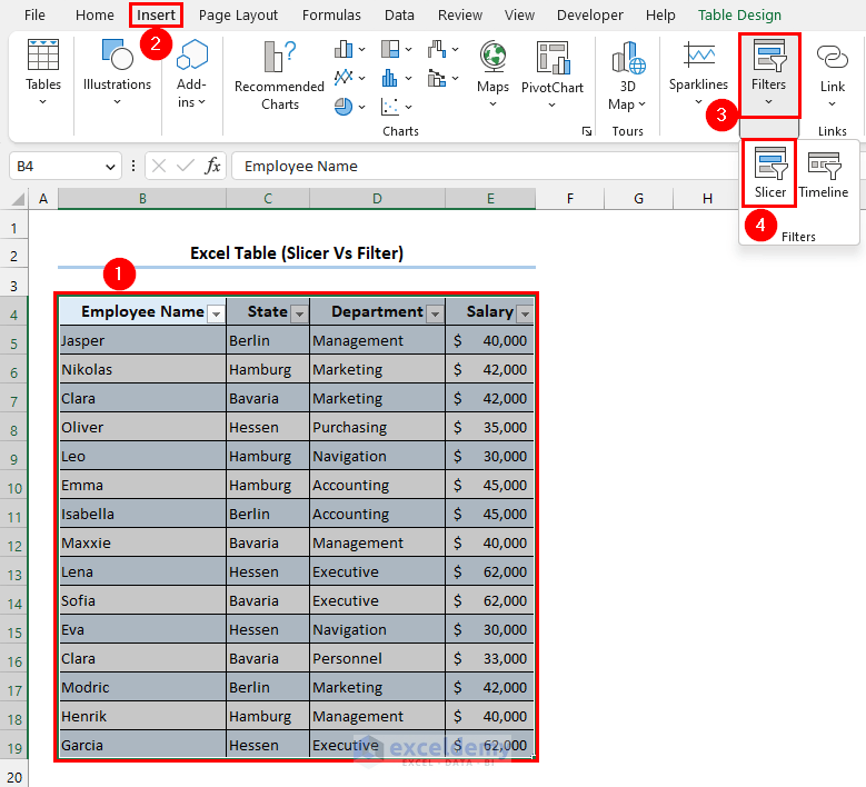
- Create a table by selecting cell range B4:E19.
- Go to the Insert tab and click on Table.
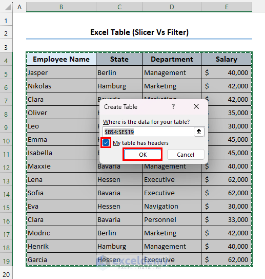
- In the Create Table dialog, mark the My table has headers option and click OK.
- Let’s filter the data:
- Using the filter feature:
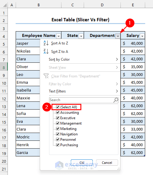
- Click the arrow down icon next to the Department header.
- Unmark the Select All box.
- Using the filter feature:
-
-
- Mark the Marketing and Executive boxes and click OK.
-

-
-
- Click the arrow down icon next to the State header.
- Unmark the Select All box and mark the Bavaria and Hessen boxes. Click OK.
-
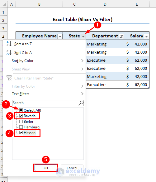
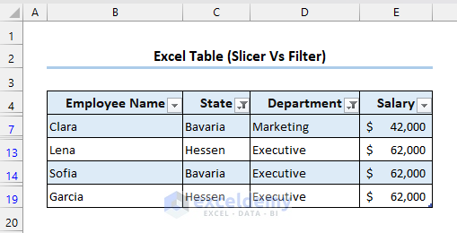
- Observe the filtered data.
Now, if we want to do the same using the slicer feature, we have to create a slicer.
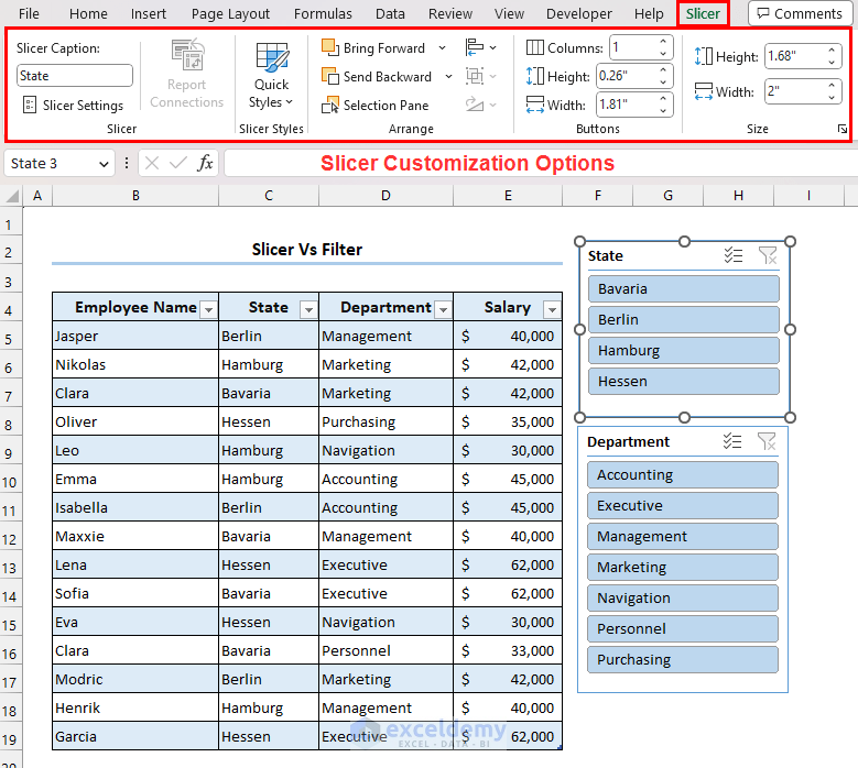
- Create a slicer by selecting the desired range (e.g., B4:E19).
- Go to the Insert tab, click on the Filters drop-down menu, and select Slicer.
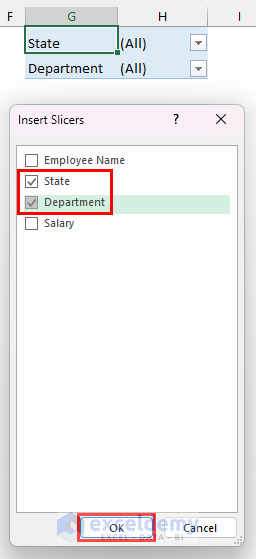
- In the Insert Slicers window, choose the fields you want to filter (e.g., State and Department).
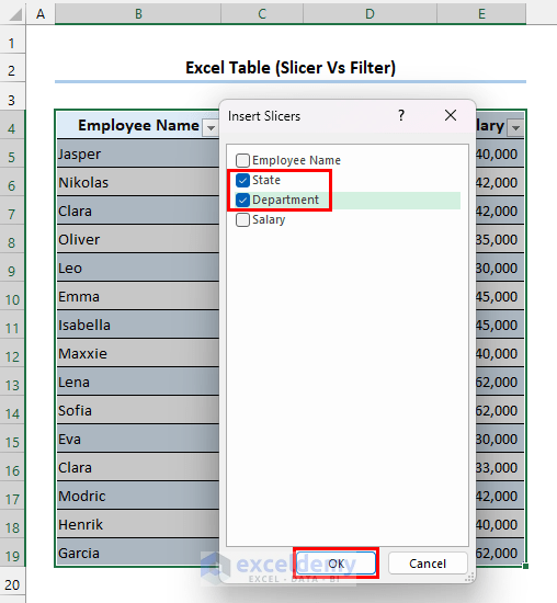
- You will see two slicers on your spreadsheet as shown below. One is titled State and the other one is titled Department.
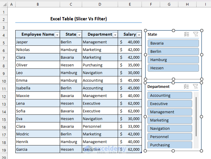
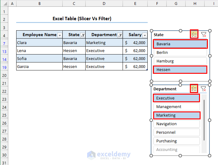
- Activate the Multi-select option.
- Select the relevant items (e.g., Bavaria, Hessen, Executive, Marketing) from the slicers.
- The filtered data will update accordingly.
2. Excel PivotTable to Explain the Difference Between Slicer and Filter
Excel PivotTable gives the opportunity to filter data using both slicer and filter features.
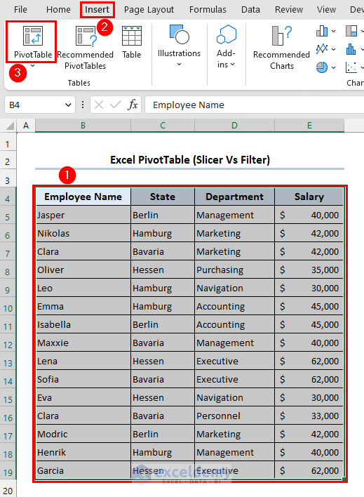
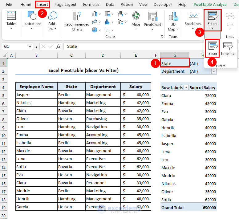
- Create a PivotTable from your dataset.
- Select cell range B4:E19.
- From the toolbar select Insert tab and click on PivotTable.
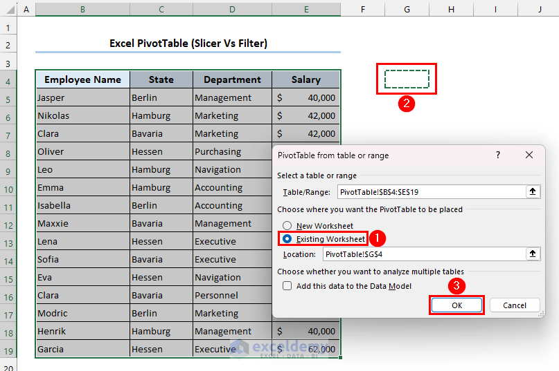
- Choose the location for the PivotTable (e.g., within the same worksheet).
- Mark the Existing Worksheet from the PivotTable from table or range dialog box.
- We have selected cell G4 as the Location to set the Pivot table.
- Click on OK.
- A sidebar tilted PivotTable Fields will appear as follows.
- Add fields to the PivotTable:
- Rows: Employee Name
- Filters: State and Department
- Values: Salary
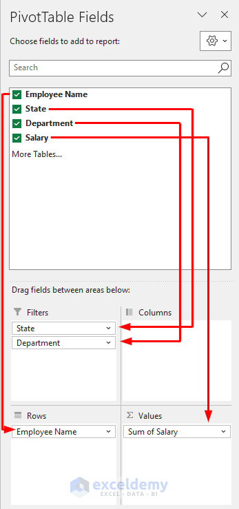
- The pivot table will be as follows.
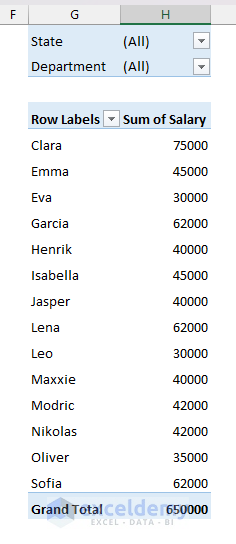
To filter data:
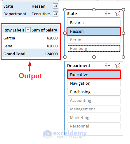
- Click the arrow down icon next to the State header (cell H1).
- Mark the Select Multiple Items box, unmark All, and select Hessen.
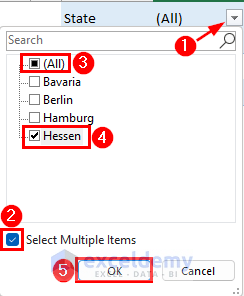
- You will see filtered data from Hessen state then.
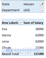
- Click the arrow down icon next to the Department header.
- Mark Select Multiple Items, unmark All, and select Executive.
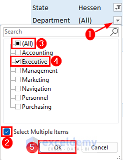
- The filtered data will be displayed in the PivotTable.
- Using Excel Slicers with PivotTable:
- Select any item from your PivotTable (e.g., the State header).
- Go to the Insert tab, click on the Filters drop-down menu, and select Slices.
- In the Insert Slicers dialog, mark the State and Department boxes, and click OK.
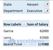
- Choose Hessen from the State slicer and Executive from the Department slicer.
- The filtered data will be shown.
3. Difference of Slicer and Filter in Excel PivotChart
Excel PivotChart is a great approach to show the differences between Excel slicer and filter. We will be using the below-modified dataset to clarify the differences between slicer and filter.
- Creating a PivotChart:
- To illustrate the differences, we’ll use a modified dataset.
- Follow these steps to create a PivotChart:
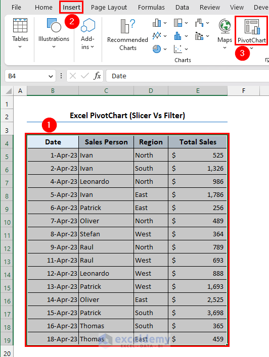
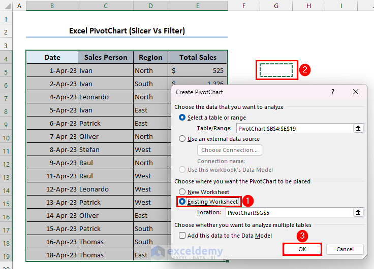
- Select the data range (e.g., B4:E19).
- Go to the Insert tab and click on PivotChart.
- Choose where you want the PivotChart (e.g., within the same worksheet).
- Mark the existing worksheet as the location (e.g., cell G5) and click OK.
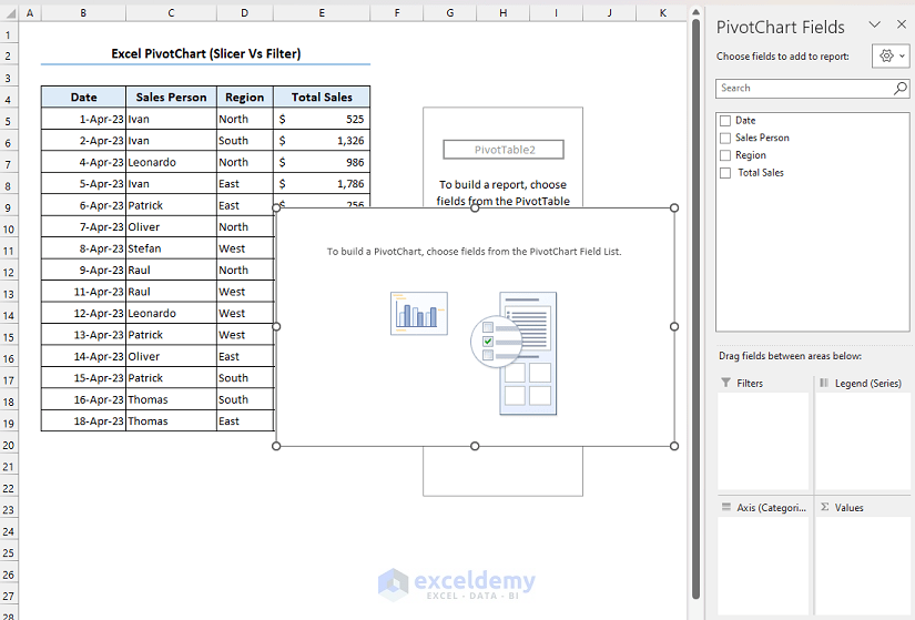
- The PivotChart Fields sidebar will appear.
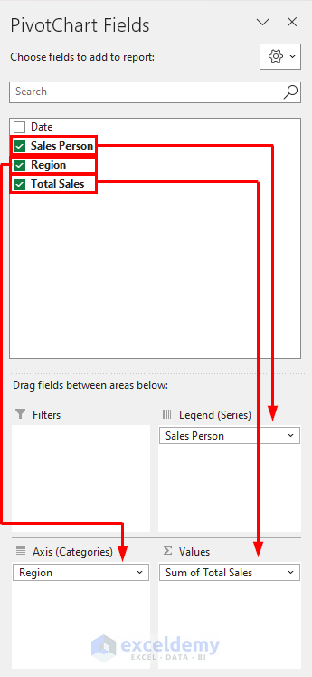
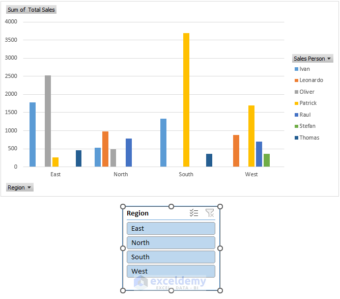
- Hold and drag the Sales Person header to the Legend (Series) field, Region header to the Axis (Categories) section, and Total Sales header to the Values field.
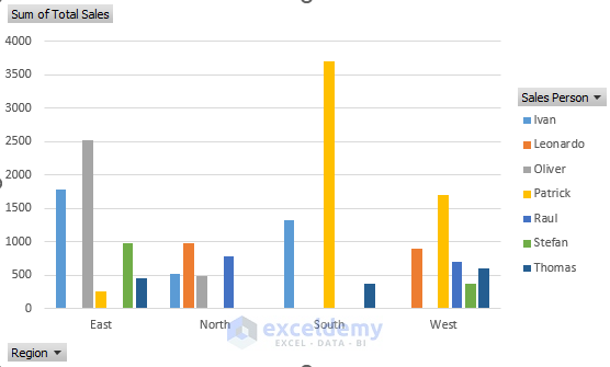
- The pivot chart will be created as follows.
- Filtering Data Using the PivotChart:
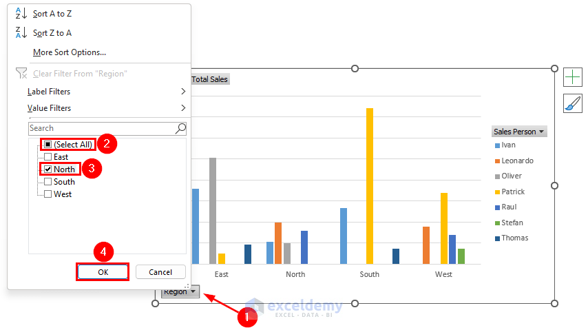
- Suppose we want to filter data for the North region in the chart.
- Click the Region drop-down menu at the bottom-left of the chart.
- Unmark the Select All box.
- Mark the North box and click OK.
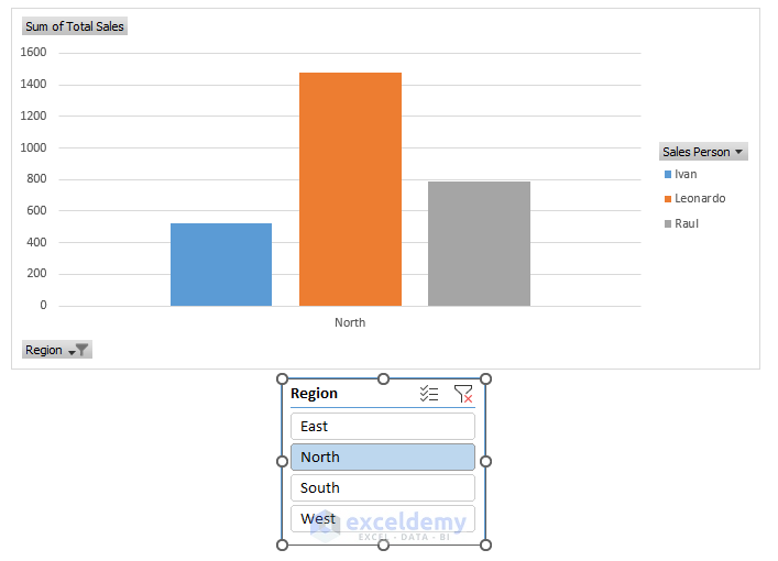
- Suppose we want to filter data for the North region in the chart.
-
-
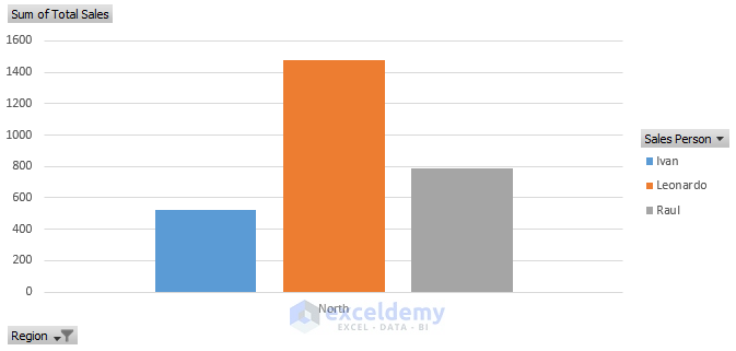
- The chart will display information for the North region only.
-
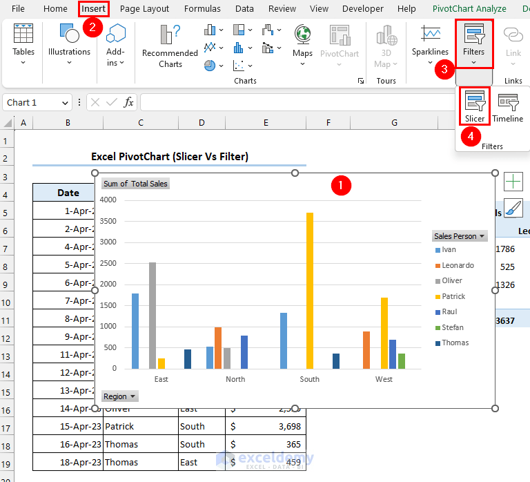
- Using Slicers with the PivotChart:
- To filter within the PivotChart using slicers:
- Select the PivotChart.
- Go to the Insert tab.
- Click on the Filters drop-down menu and choose Slicer.
- To filter within the PivotChart using slicers:
-
-
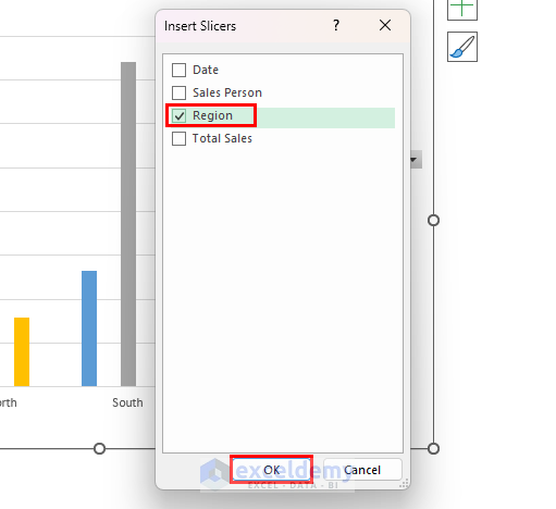
- In the Insert Slicers dialog, mark the Region box and click OK.
-
-
-
- The slicer will be created.
- You can now filter data within the chart using this slicer.
-
- Select the North option from the slicer to show data from the North region.
- The chart will show data from the North region only as follows.
Excel Slicer Vs Filter: Advantages and Disadvantages
The major advantages and disadvantages of Excel slicer and filter can be measured based on various indicators. Some of these are described below.
Application of Slicer and Filter
Slicer
- Requires creating a table or pivot table.
Filter
- Default feature in Excel.
- Available for Excel Table, PivotTable, and PivotChart.
- Select any header cell.
- Go to the Home tab in the toolbar.
- Click on the Editing drop-down menu.
- Select Filter from Sort & Filter section.
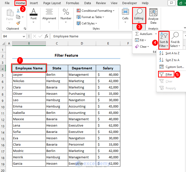
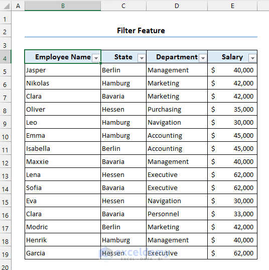
- The Filer Feature will be available for your dataset.
Filtering Options in Excel
Slicer:
- Limited filtering options compared to Excel’s Filter feature.
Filter
- Offers more extensive filtering options.
User Interface of Slicer and Filter in Excel
- Slicer:
- Aesthetically pleasing and engaging interface.
- Filter:
- Uses a drop-down menu or dialog box.
Customization of Slicer
- Slicer:
- Customizable (e.g., color, button arrangement, dimensions, header).
- Filter:
- Limited customization.
Read More: How to Custom Sort Slicer in Excel
Formatting Excel Slicers
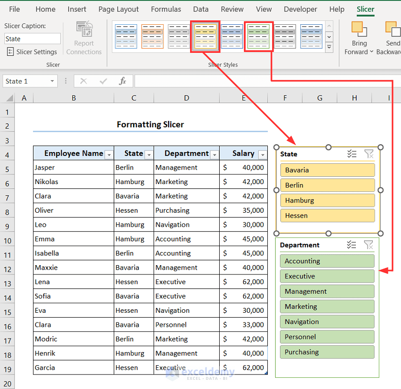
1. Changing Colors
- After inserting a slicer, you’ll find a new tab called Slicer in the toolbar.
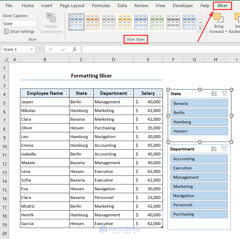
- In the Slicer Styles section, you can easily change the colors of your slicers.
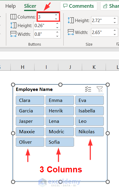
2. Adding Multiple Columns
- You can rearrange the buttons within your slicer to display them in multiple columns.
- In the Slicer tab, locate the Buttons section.
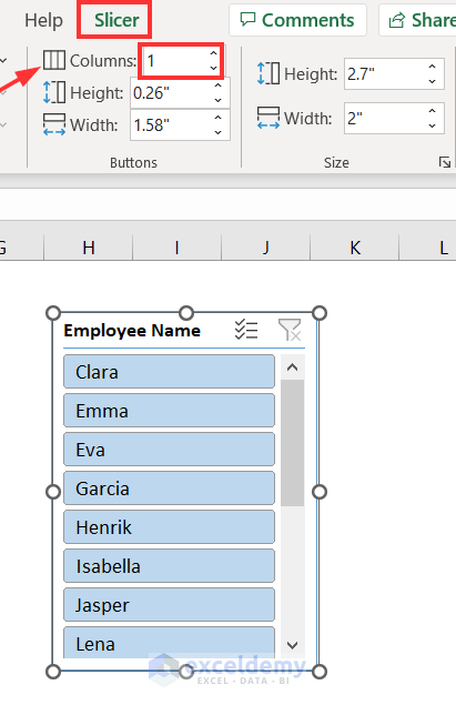
- Modify the column count by typing the desired number (e.g., 3) in the Columns box.
- And the output will be as follows.
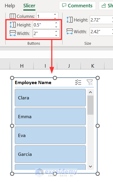
3. Modifying Buttons
- Adjust the dimensions of the slicer buttons for better visualization.
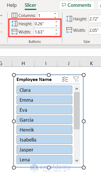
- In the Buttons section, set the height to 0.5 inches and the width to 2 inches.
- Now your buttons will appear larger.
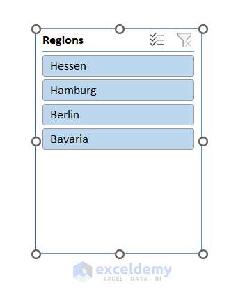
4. Slicer Settings
- Slicer settings allow you to customize the appearance and functionality of these visual tools.
- Right-click on your slicer and select Slicer Settings.
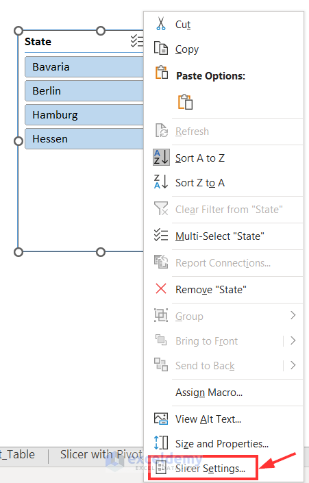
- In the Slicer Settings dialog box, you can modify the slicer name, title, and other settings.
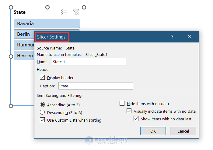
- For example, set the slicer name to Regions, the header to Regions, sort buttons in descending order, and hide items with no data.
- Click OK to apply the changes.
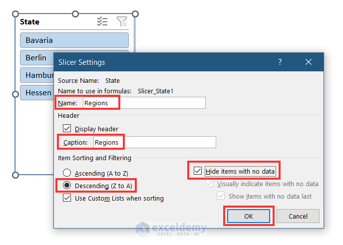
- And the slicer will be as follows.
Frequently Asked Questions
- Which Is Better: Slicer or Filter?
- Slicers are more beneficial when you want users to interactively explore data in real-time.
- Filters are useful for limiting data based on predefined criteria.
- The choice depends on your specific needs.
- Is a Slicer a Filter in Excel?
- Yes, a slicer is a type of filter in Excel.
- It provides a visual interface for customizing data in pivot tables, pivot charts, or Excel tables.
- Which Is Faster: Slicer or Filter?
- Generally, both slicers and filters process data efficiently.
- Performance differences depend on factors like data volume, complexity, and computer speed.
- Do Slicers Slow Down Excel?
- Excel slicers are designed for speed and won’t significantly slow down your workbook.
- Performance may vary based on data size and slicer usage.
- Why Are Slicers Better Than Report Filters?
- Slicers offer dynamic, user-friendly data filtering.
- They allow simultaneous filtering across multiple fields and enhance dashboard aesthetics.
- While report filters have advantages, slicers are often more effective.
Download Practice Workbook
You can download the practice workbook from here:
Further Readings
- How to Create Slicer Drop Down in Excel
- How to Make Excel Slicer with Search Box
- How to Create Timeline Slicer with Date Range in Excel

