Advanced Filter with Multiple Criteria in Excel (15 Suitable Examples)

Example 1 – Advanced Filter for AND Criteria

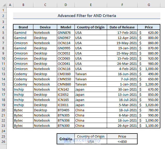
Below is our sample dataset. We’re going to extract data for all devices made in the USA and devices with prices less than $850.

Step 1:

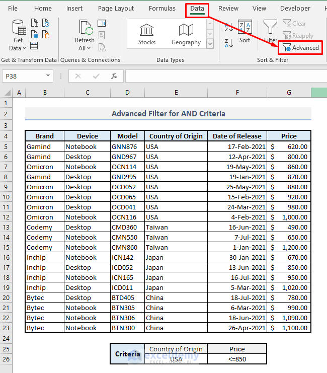
➤ From the Data tab, go to the Sort & Filter group of commands and select the Advanced command. A dialogue box will appear.

Step 2:

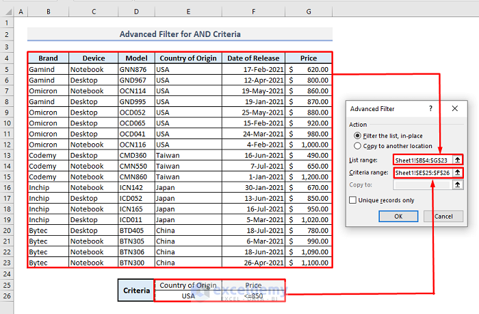
➤ For List Range, select the entire array or the table(B4:G23).

➤ Select the criteria array(E25:F26) for Criteria Range.

➤ Press Ok.

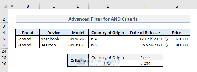
Result will show the filtered data according to the selected criteria.

To use Advanced Filter effectively, you have to select the criteria with two rows at least or it won’t work. For the criteria section in the spreadsheet, you have to use headers for the related columns where filtering criteria will be applied. Advanced Filter will search for the selected criteria under that defined header from the criteria section in your Excel sheet.

Example 2 – Advanced Filter for OR Criteria

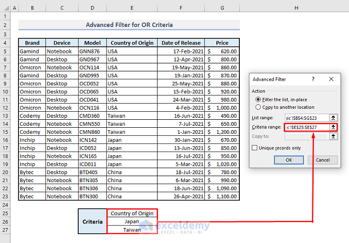
We will filter with OR criteria, that means two different criteria will be applied to one single column. Assuming that we want to filter the table for the devices made in Japan and Taiwan only. In the criteria section(E25:E27), Japan and Taiwan are in a column under the Country of Origin header. You have to add criteria in a column under the related header for OR logic.

Steps:

➤ The List Range will occupy the range of cells- B5:G23.

➤ Select the range of cells E25:E27 for the Criteria Range.

➤ Press OK.

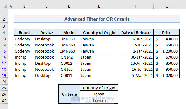
You will get the filtered result as shown in the following image.

Example 3 – Advanced Filter for AND-OR Criteria

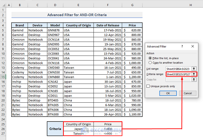
We can combine both AND and OR criteria in Advanced Filter. Based on our dataset, we will add two different criteria in two columns and filter the data for the devices made in Japan that cost not more than $800 and the devices made in Taiwan that cost not more than $900.

List Range: B4:G23

Criteria Range: E25:F27

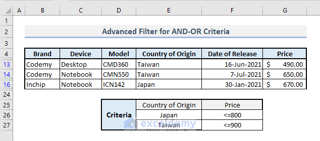
The filtered output is shown in the following image.

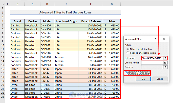
Example 4 – Advanced Filter to Show Unique Rows

The sample dataset has been modified for this section. There are a number of duplicate rows in the table that I have highlighted with different colors. We will filter the entire data to show all rows without duplications.

List Range: B4:G23

Criteria Range: (You don’t need to define here now)

Put a checkmark on the Unique Records option and press OK.

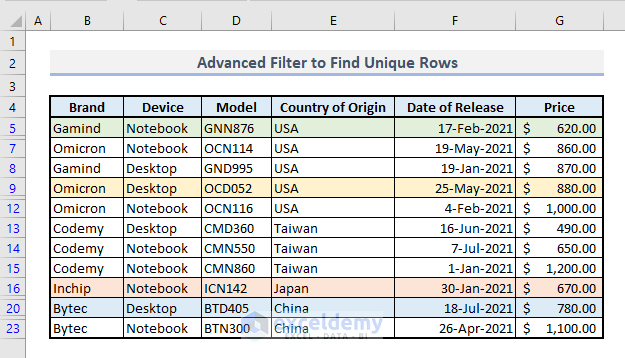
You will find the filtered table with all unique rows without any duplicate.

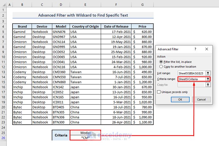
Example 5 – Advanced Filter with Wildcards to Find Specific Texts

There are 3 types of wildcard characters in Excel- 

? (Question Mark) – Represents any single character in a text.

* (Asterisk) – Represents any number of characters.

~ (Tilde) – Represents the presence of a wildcard character in the text.

By using Asterisk(*) before and after a text in the criteria section, we can search for a specific text string in our table. We’re going to find the text “CM” in the column of Model names.

List Range: B4:G23

Criteria range: E25:E26

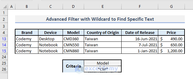
As shown in the image below, you will get the model names with ‘CM’ text inside. By using Asterisks before & after ‘CM’, we are simply rendering the information to the Excel function that there might be more texts before or after ‘CM’ and thus the function follows the command to show the exact output from the range of cells or an array.

Example 6 – Advanced Filter for Case-Sensitive Texts

To filter a table with case-sensitive texts, we have to enter a formula manually to execute the function for the 1st row and this formula or function must return with logical values and input this logical value along with a random header in the Criteria Range of the Advanced Filter box.

NOTE: When applying a logical function manually for the 1st row, the header for this criteria must not match with any of the headers present in the original dataset or table.

The formula to find case-sensitive text in Cell E26 is:

List Range: B4:G23

Criteria range: E25:E26

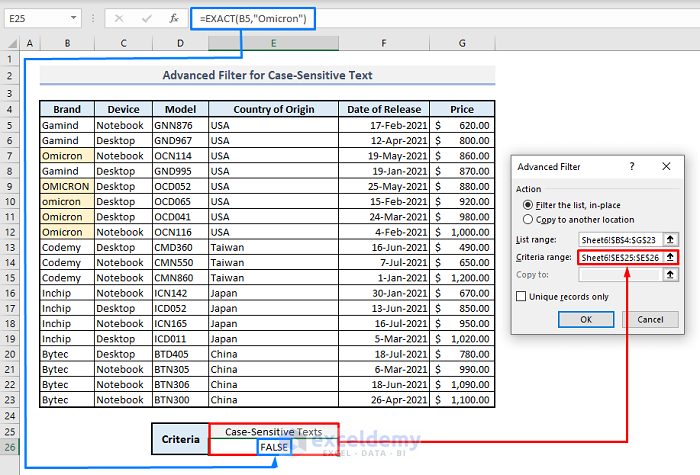
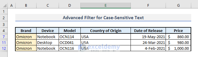
There are 5 names with ‘Omicron’ in Column B but they are not case-sensitive. As we’ll extract the data based on exactly ‘Omicron’ with case-sensitive active, follow the steps mentioned above to get the filtered table as shown below.

Read More: How to Use Advanced Filter If Criteria Range Contains Text in Excel

Example 7 – Advanced Filter for Calculated Results

We will find out the devices that cost more than the average price of all values from Column G. Enter a logical function in Cell E26 for the 1st row that will indicate if the price mentioned in the 1st row is more than the average of all prices or not. The related function will be:

List Range: B4:G23

Criteria Range: E25:E26

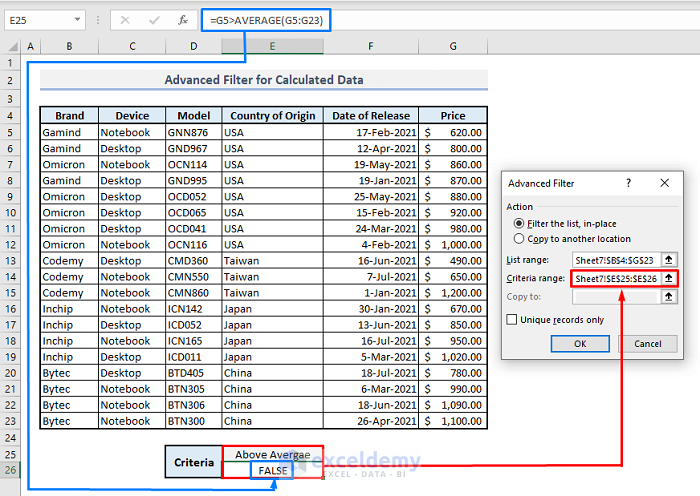
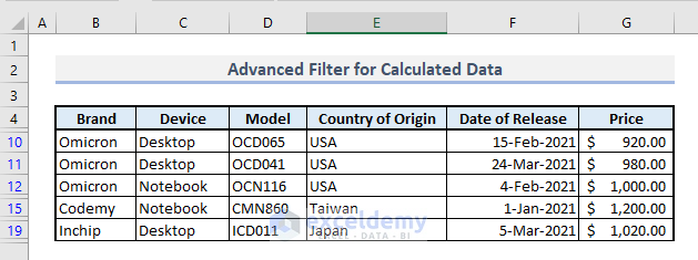
You’ll get the following result.

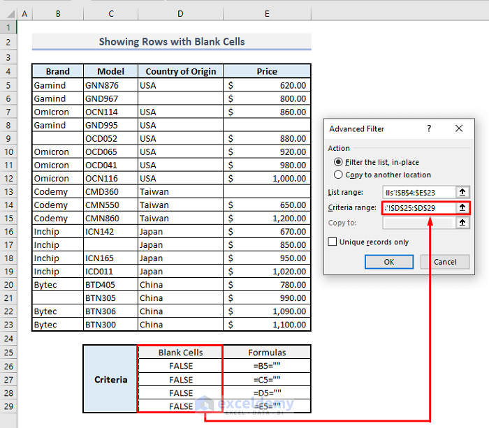
Example 8 – Advanced Filter to Show Rows with Blank Cells

In our sample dataset below, there are some blank cells. Using Advanced Filter, extract those rows containing blank cells. In Column E under the table, the formulas to find blank cells for all columns is mentioned. And the left column with Blank Cells header represents the criteria range for the Advanced Filter option.

List Range: B4:E23

Criteria Range: D25:D29

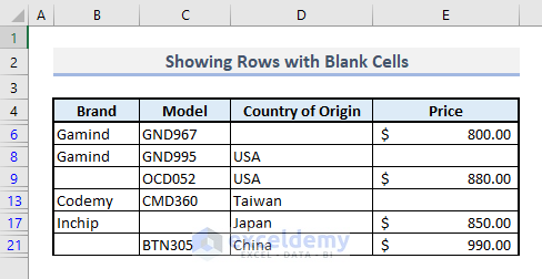
Filter the table with the selected criteria to get the following results with all rows containing blank cells.

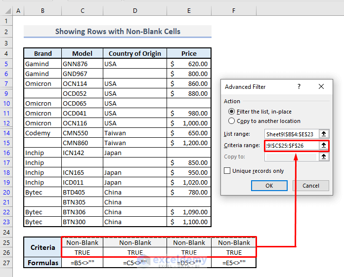
Example 9 – Advanced Filter to Show Rows with Non-Blank Cells

To extract the rows with non-blank cells and the criteria has to be applied to 4 different columns separately, use AND logic. Add the criteria for 4 columns in a row, not in a column. , You will find the formulas that have been used to find return values under the logical values.

List Range: B4:E23

Criteria Range: C25:F26

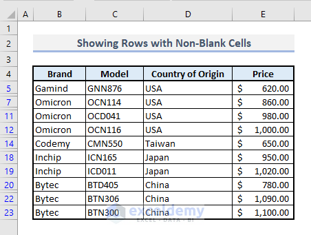
The following image is the filtered output under the mentioned criteria.

Example 10 – Advanced Filter to Find Top 5 Values

To find the top 5 values from a range of cells with numeric values, enter a formula that will search for the value equal to or larger than the 5th largest values from the Price column. The related logical function in Cell D26 will be:

List Range: B4:F23

Criteria Range: D25:E26

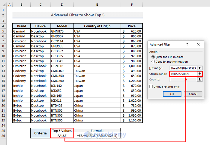
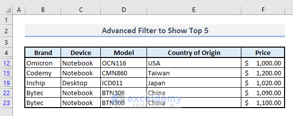
The output data with the top or highest 5 numerical values will be as shown in the image below.

Example 11 – Advanced Filter to Find Bottom 5 Values

Enter the following formula in Cell D26:

List Range: B4:F23

Criteria Range: D25:E26

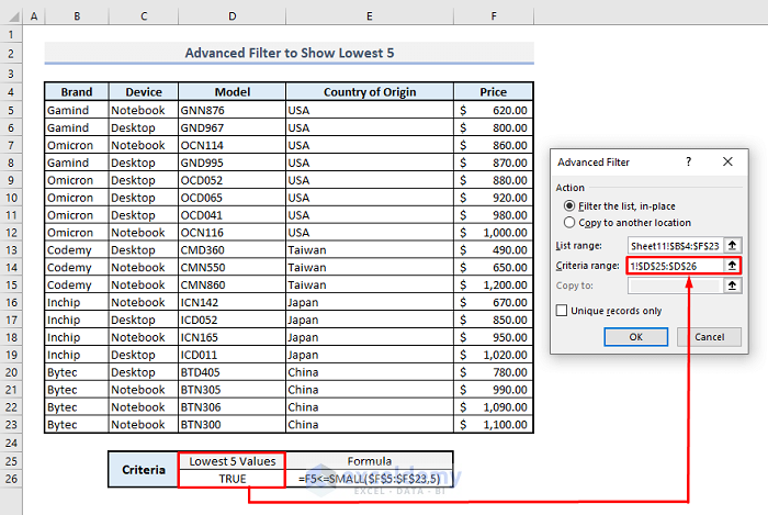
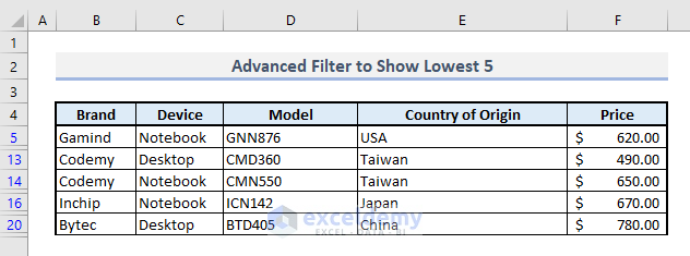
Advanced Filter to get the following result with the bottom or lowest 5 numerical values from the Price column.

Example 12 – Advanced Filter for Matches in the Same Rows

The sample dataset below contains two columns with the model names of computer devices. To find the matches in similar rows and extract the filtered data with Advanced Filter, enter the following formula in Cell C26,

List Range: B4:C23

Criteria Range: C25:C26

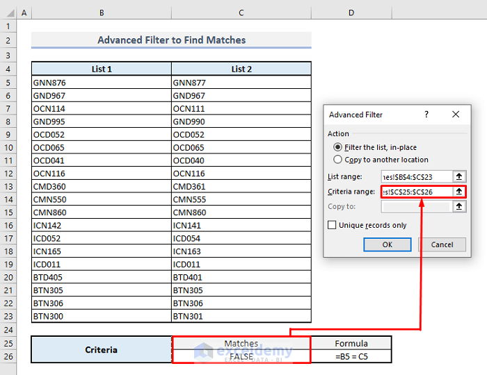
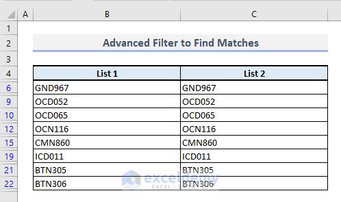
The filtered result will look like in the following image:

Example 13 – Advanced Filter for Differences Along Similar Rows

To find the differences in the similar row between two columns, we have to use the ‘Not Equal To’(<>) symbol between two cells for logical function. Enter the following formula in Cell C26,

List Range: B4:C23

Criteria Range: C25:C26

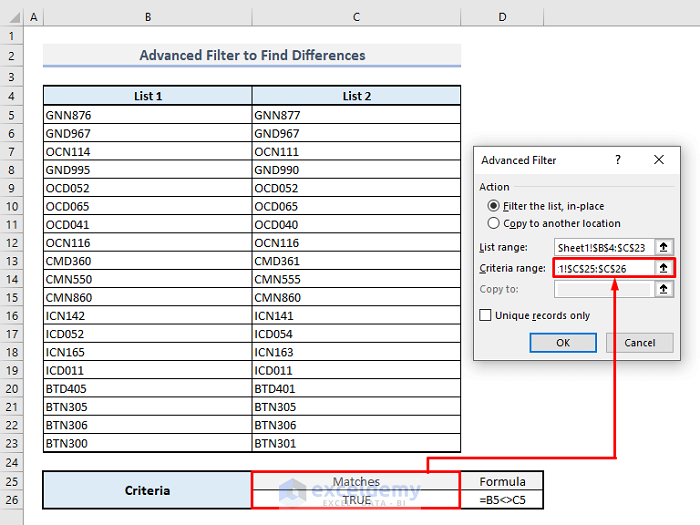
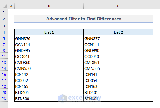
The filtered result for the rows with different texts alongside is shown below.

Example 14 – Advanced Filter to Find Weekdays

In the sample dataset below, there are two columns with a number of product ID’s along with the assigned delivery dates. We will filter the dates that include the weekdays only considering the weekends as Saturday & Sunday.

Enter the following formula in Cell C26,

List Range: B4:C23

Criteria Range: C25:C26

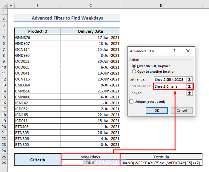
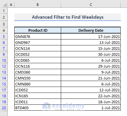
We are adding two different weekday numbers for Saturday & Sunday with AND function. By default, in WEEKDAY function, Sunday starts with 1 & Saturday ends with 7 as weekday numbers. By entering a logical function that will not be equal to these two weekday numbers, we can filter the weekdays easily. The following image is the filtered data found through the Advanced Filter.

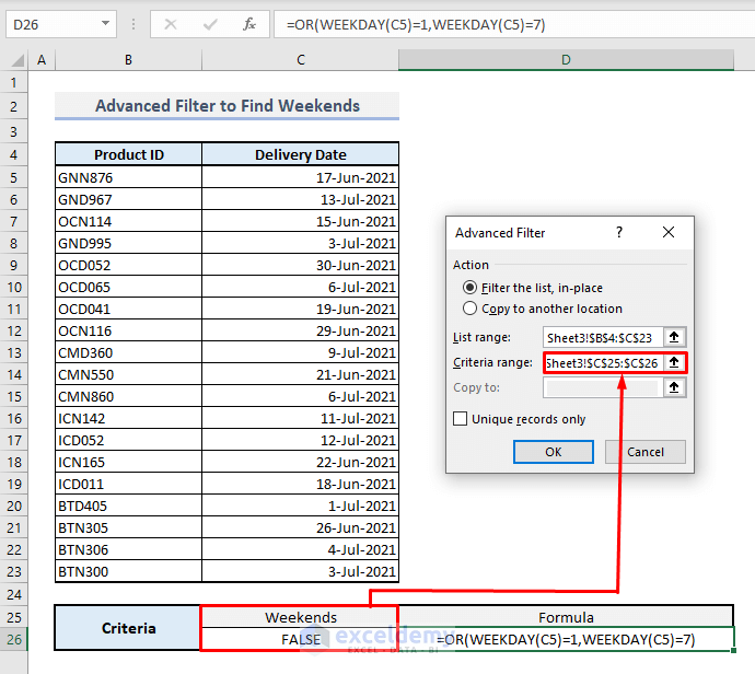
Example 15 – Advanced Filter to Filter Weekends

Enter the following formula in Cell C26:

List Range: B4:C23

Criteria Range: C25:C26

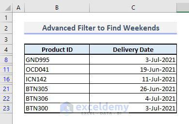
You’ll get the filtered results with weekends.

Download Practice Workbook

<< Go Back to Advanced Filter | Filter in Excel | Learn Excel